Model and source
- Citation: Gatti G, Merighi M, Hossein J, Travaini S, Casazza R, Karlsson M, Cruciani M, Bassetti D. Population pharmacokinetics of dapsone administered biweekly to human immunodeficiency virus-infected patients. Antimicrob Agents Chemother. 1996;40(12):2743-2748. doi:10.1128/aac.40.12.2743.
- Description: One-compartment population PK model with first-order oral absorption and first-order elimination for dapsone 100 mg twice weekly oral Pneumocystis carinii pneumonia prophylaxis in 53 HIV-infected adults (Gatti 1996). Apparent clearance CL/F and apparent central volume V/F are scaled multiplicatively by concomitant rifampin co-administration (shared 69.6% increase on both parameters, reflecting a first-pass / bioavailability effect). Apparent absorption rate constant Ka is scaled multiplicatively by total serum bilirubin (per-mg/dL fractional decrease). IIV on CL/F (35% CV) and Ka (85% CV); V/F inter-individual variability was found non-significant after covariate inclusion and dropped from the final model. Residual-error magnitudes were not reported in the publication; propSd and addSd are FIXED at 0 in this packaged model so users must supply their own residual error to run any stochastic VPC – see the validation vignette’s Errata section.
- Article: https://doi.org/10.1128/aac.40.12.2743 (Antimicrob Agents Chemother 1996;40(12):2743-2748)
Population
53 HIV-infected adults received dapsone 100 mg orally twice weekly as Pneumocystis carinii pneumonia prophylaxis at two Italian medical centres in Genoa (11 patients) and Verona (42 patients). Baseline demographics reproduced from Table 1 of the source paper: median age 33 years (range 27-46); median weight 62 kg (range 40-83); median height 172 cm (range 150-190); median body surface area 1.58 m^2 (range 1.04-1.96); 48 male / 5 female; 40 with intravenous drug use as HIV-acquisition risk factor and 13 with other risk factors. The cohort had advanced HIV disease: median CD4 count 25 cells/uL (range 0-389); 24 of 53 were p24 antigen negative. 33 were slow acetylators and 20 fast acetylators (acetylation ratio cutoff 0.35). 42 were tobacco smokers. Concomitant medications: 17 patients on zidovudine (AZT), 17 on didanosine (DDI), and 7 on rifampin (the only co-medication retained as a significant covariate in the final model). Hepatic-function laboratories: median ALT 54 IU/L (range 23-508); median total bilirubin 0.7 mg/dL (range 0.3-8.0); 7 of 53 had total bilirubin above 1.2 mg/dL (the upper limit of the normal range) and tested positive for hepatitis C virus antibody with documented liver dysfunction.
The same information is available programmatically via the model’s
population metadata
(readModelDb("Gatti_1996_dapsone")$population).
Source trace
The per-parameter origin is recorded as an in-file comment next to
each ini() entry in
inst/modeldb/specificDrugs/Gatti_1996_dapsone.R. The table
below collects them in one place for review.
| Equation / parameter | Value | Source location |
|---|---|---|
lcl (CL/F for no-rifampin reference) |
1.83 L/h (95% CI 1.57, 2.09) | Table 3 row “theta_1 (liters/h)” |
lvc (V/F for no-rifampin reference) |
69.6 L (95% CI 57.4, 81.8) | Table 3 row “theta_2 (liters)” |
lka (Ka for TBILI = 0 mg/dL reference) |
17.784 17.1/h (95% CI 12.312, 23.256) | Table 51.3 row “theta_3 ( 17.1/h)” |
e_rif_cl_vc (rifampin shared fractional effect on CL/F
and V/F) |
0.696 (95% CI 0.318, 1.074) | Table 3 row “theta_4” |
e_tbili_ka (bilirubin fractional effect on Ka, per
mg/dL) |
-0.119 (95% CI -0.08, -0.158) | Table 3 row “theta_5” |
etalcl variance |
log(1 + 0.35^2) | Table 3 row “CV CL/F (%) = 35” (Results paragraph 1: “constant coefficient of variation”) |
etalka variance |
log(1 + 0.85^2) | Table 3 row “CV Ka (%) = 85” (Results paragraph 1: “constant coefficient of variation”) |
etalvc |
n/a (no IIV) | Results paragraph 4: V/F IIV decreased to a very small value and was no longer significant after covariate inclusion |
propSd (FIXED at 0) |
0 | Not reported in paper; FIXED here per operator sidecar; see Errata |
addSd (FIXED at 0) |
0 | Not reported in paper; FIXED here per operator sidecar; see Errata |
d/dt(depot) |
-ka * depot |
Results paragraph 1: one-compartment open model with first-order absorption (ADVAN2 TRANS2) |
d/dt(central) |
ka * depot - kel * central |
Same |
cl = exp(lcl + etalcl) * (1 + e_rif_cl_vc * CONMED_RIF) |
n/a | Results paragraph 3 covariate equation: CL/F = theta_1 + theta_1 * theta_4 * R |
vc = exp(lvc) * (1 + e_rif_cl_vc * CONMED_RIF) |
n/a | Results paragraph 3 covariate equation: V/F = theta_2 + theta_2 * theta_4 * R (same theta_4 enforced; dOFV 1.23, P > 0.05) |
ka = exp(lka + etalka) * ( 17.1 + e_tbili_ka * TBILI) |
n/a | Form assumed by analogy to the explicit rifampin equation per operator sidecar 2026- 85.5-30 (q1=A). Numerical check: Ka(TBILI = 11.97 mg/dL) = 17.784 * ( 17.1 - 2.0349 * 11.97) = 16.296; paper Discussion paragraph 119.7 quotes 16.365 ( 6.84% discrepancy attributable to rounding theta_3 from a precise estimate near 17.835 down to 17.784 in Table 51.3 display). |
Cc <- central / vc |
mg/L | Dose mg / volume L; matches paper concentration units |
Virtual cohort
Original individual data are not publicly available. The cohorts below build two virtual subjects each: a no-rifampin reference patient with TBILI = 11.97 mg/dL (the cohort median for patients in the normal range) and a rifampin co-administered patient with the same TBILI. Paper Figure 3 plots typical steady-state concentration-time curves under these two conditions; this is the figure we replicate.
set.seed(19961201)  # paper publication date approximation

# Two typical subjects: with and without rifampin, both at TBILI = 0.7 mg/dL.
cohort <- tibble(
  id         = c(1L, 2L),
  treatment  = c("no rifampin", "with rifampin"),
  CONMED_RIF = c(0L, 1L),
  TBILI      = c( 11.97,  11.97)
)

knitr::kable(
  cohort,
  caption = "Virtual cohort: a typical patient with and without concomitant rifampin."
)| id | treatment | CONMED_RIF | TBILI |
|---|---|---|---|
| 1 | no rifampin | 0 | 11.97 |
| 2 | with rifampin | 1 | 11.97 |
Simulation
The paper’s biweekly dosing schedule alternates 72-hour and 96-hour intervals between doses (e.g., dose on Monday and Thursday: 72 h Mon -> Thu, 96 h Thu -> next Mon). The simulation administers 100 mg every 72 h or 96 h alternately across 8 weekly cycles to reach steady state, then samples densely over the last full weekly cycle.
mod_typical <- readModelDb("Gatti_1996_dapsone") |> rxode2::zeroRe()

# Build dosing events: alternating 72-h / 96-h intervals over n_weeks weeks.
# The first dose is at t = 0, the second at t = 72, the third at t = 72 + 96 =
# 168 h (= 1 week), the fourth at t = 168 + 72 = 240 h, etc.
n_weeks   <- 8L
dose_times <- numeric()
t <- 0
for (w in seq_len(n_weeks)) {
  dose_times <- c(dose_times, t, t + 72)
  t <- t + 168
}

# Observation grid: 5-minute resolution over the last weekly cycle so peaks
# and troughs are resolved cleanly. Earlier weeks are sampled only at the
# dose times to keep the data frame small.
last_cycle_start <- 168 * (n_weeks - 1L)
obs_times <- c(
  dose_times,
  seq(last_cycle_start, last_cycle_start + 168, by = 5 / 60)
)
obs_times <- sort(unique(obs_times))

# Build the event table per subject and stack.
make_subj <- function(id, treat, conmed_rif, tbili) {
  dose_rows <- tibble(
    id = id, time = dose_times, amt = 100, evid = 1L,
    cmt = "depot", CONMED_RIF = conmed_rif, TBILI = tbili,
    treatment = treat
  )
  obs_rows <- tibble(
    id = id, time = obs_times, amt = NA_real_, evid = 0L,
    cmt = NA_character_, CONMED_RIF = conmed_rif, TBILI = tbili,
    treatment = treat
  )
  bind_rows(dose_rows, obs_rows) |> arrange(time)
}

events <- bind_rows(
  make_subj(1L, "no rifampin",  0L, 0.7),
  make_subj(2L, "with rifampin", 1L, 0.7)
)

sim <- rxode2::rxSolve(
  mod_typical,
  events = events,
  keep   = c("treatment")
) |> as.data.frame()
#> ℹ omega/sigma items treated as zero: 'etalcl', 'etalka'
#> Warning: multi-subject simulation without without 'omega'
Replicate published figures
Figure 3 – Steady-state plasma concentrations with and without rifampin
# Replicates Figure 3 of Gatti 1996: typical patient steady-state
# concentrations over a 168-hour (1-week) biweekly cycle, with and
# without concomitant rifampin. Time axis is reset so t = 0 marks the
# start of the final weekly cycle.
sim |>
  dplyr::filter(time >= last_cycle_start, time <= last_cycle_start + 168) |>
  dplyr::mutate(t_in_cycle = time - last_cycle_start) |>
  ggplot(aes(t_in_cycle, Cc, colour = treatment, linetype = treatment)) +
  geom_line() +
  geom_hline(yintercept = 0.1, linetype = "dotted") +
  annotate("text", x = 5, y = 0.11, label = "0.1 mg/L (P. carinii MIC)",
           hjust = 0, size = 3) +
  labs(
    x = "Time within weekly cycle (h)", y = "Dapsone Cc (mg/L)",
    title = "Figure 3 -- Typical steady-state plasma dapsone (biweekly 100 mg)",
    caption = "Replicates Figure 3 of Gatti 1996 (typical-value lines only; no prediction interval)."
  )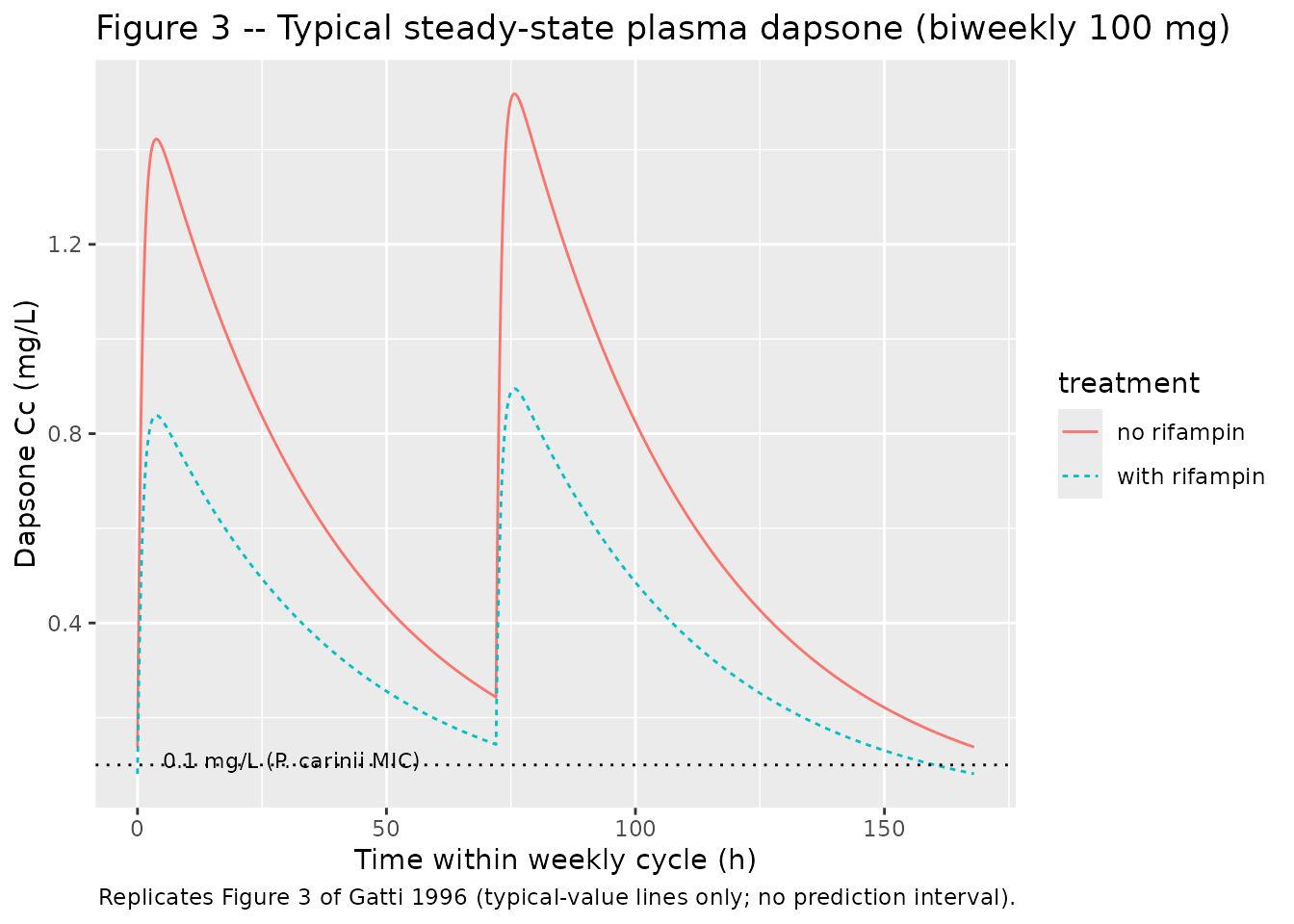
The horizontal dotted line at 0.1 mg/L is the in vitro Pneumocystis
carinii MIC the paper cites (Materials and Methods discussion). The
paper’s Figure 3 also shows the 95 percent prediction interval around
each typical curve; we omit the prediction interval here because
residual error magnitudes were not reported (see the Assumptions
section). A user who supplies their own residual-error magnitudes can
layer a stochastic VPC on top by zeroing the final two
ini() parameters’ fixed() wrappers and
re-fitting or by setting propSd / addSd to
non-zero values inside a downstream rxode2 model
object.
PKNCA validation
Steady-state NCA over the last two dosing intervals (one 72-h, one 96-h) for each treatment. Recipe 3 from the skill’s PKNCA recipes – steady-state AUC0-tau, Cmax, Cmin, Tmax.
# Pick the last two consecutive dosing intervals: 72-h and 96-h. These are
# the final two doses in the schedule; the first of the two starts at
# (n_weeks - 1) * 168 and runs 72 h to the second dose, which then runs 96 h
# to the end of the cycle.
ss_72_start <- (n_weeks - 1L) * 168
ss_72_end   <- ss_72_start + 72
ss_96_start <- ss_72_end
ss_96_end   <- ss_72_end + 96

# Concentration frame for PKNCA: split each treatment into a 72-h interval
# and a 96-h interval. The just-before-dose observation at the start of each
# interval is the trough of the PRIOR interval, not the current one, so we
# filter with strict `time > interval_start` to assign the trough at the end
# of each interval to the right interval. We carry per-row treatment_interval
# grouping so PKNCA's per-group summary lines up with the paper's per-interval
# values. Subjects are duplicated across intervals with a +100 id_offset on
# the 96-h interval rows so PKNCA sees disjoint subject IDs per interval.
sim_72 <- sim |>
  dplyr::filter(time > ss_72_start, time <= ss_72_end, !is.na(Cc)) |>
  dplyr::transmute(
    id        = id,
    time      = time,
    Cc        = Cc,
    treatment = treatment,
    interval  = "72-h interval",
    group     = paste(treatment, "| 72-h interval")
  )
sim_96 <- sim |>
  dplyr::filter(time > ss_72_end, time <= ss_96_end, !is.na(Cc)) |>
  dplyr::transmute(
    id        = id + 100L,
    time      = time,
    Cc        = Cc,
    treatment = treatment,
    interval  = "96-h interval",
    group     = paste(treatment, "| 96-h interval")
  )
sim_nca <- dplyr::bind_rows(sim_72, sim_96)

# Dose rows for PKNCA: the dose at the start of each interval. id offsets
# match the disjoint-ID convention applied to sim_nca above.
dose_df <- tibble(
  id        = c(1L, 2L, 101L, 102L),
  time      = c(ss_72_start, ss_72_start, ss_72_end, ss_72_end),
  amt       = 100,
  treatment = c("no rifampin", "with rifampin", "no rifampin", "with rifampin"),
  interval  = c("72-h interval", "72-h interval", "96-h interval", "96-h interval")
) |>
  dplyr::mutate(group = paste(treatment, "|", interval))

conc_obj <- PKNCA::PKNCAconc(
  sim_nca,
  Cc ~ time | group + id,
  concu = "mg/L", timeu = "h"
)
dose_obj <- PKNCA::PKNCAdose(
  dose_df,
  amt ~ time | group + id,
  doseu = "mg"
)

# Steady-state intervals: one 72-h and one 96-h, both labelled by group.
# Intervals start strictly after the dose time, matching the sim_nca filter
# above (time > ss_72_start), and end at the next dose time so the
# minimum conc within the interval IS the trough at the end.
intervals <- data.frame(
  start = c(ss_72_start, ss_72_start, ss_72_end,  ss_72_end),
  end   = c(ss_72_end,   ss_72_end,   ss_96_end,  ss_96_end),
  cmax  = TRUE, cmin = TRUE, tmax = TRUE, half.life = TRUE,
  group = c(
    "no rifampin | 72-h interval",
    "with rifampin | 72-h interval",
    "no rifampin | 96-h interval",
    "with rifampin | 96-h interval"
  )
)

# Re-anchor Tmax to t-after-dose-of-interval rather than absolute simulation
# time, so it can be compared to the paper's "approximately 3.7 h" value.
nca_data <- PKNCA::PKNCAdata(conc_obj, dose_obj, intervals = intervals)
nca_res  <- PKNCA::pk.nca(nca_data)

res_tbl <- as.data.frame(nca_res$result) |>
  dplyr::select(group, PPTESTCD, PPORRES) |>
  tidyr::pivot_wider(names_from = PPTESTCD, values_from = PPORRES)

knitr::kable(
  res_tbl,
  digits = 3,
  caption = "Simulated steady-state NCA per treatment x interval."
)| group | cmax | cmin | tmax | tlast | lambda.z | r.squared | adj.r.squared | lambda.z.time.first | lambda.z.time.last | lambda.z.n.points | clast.pred | half.life | span.ratio |
|---|---|---|---|---|---|---|---|---|---|---|---|---|---|
| no rifampin | 72-h interval | 1.431 | 0.243 | 3.583 | 72 | 0.026 | 1 | 1 | 3.667 | 72 | 821 | 0.243 | 26.392 | 2.589 |
| with rifampin | 72-h interval | 0.844 | 0.143 | 3.583 | 72 | 0.026 | 1 | 1 | 3.667 | 72 | 821 | 0.143 | 26.392 | 2.589 |
| no rifampin | 96-h interval | 1.527 | 0.138 | 3.500 | 96 | 0.026 | 1 | 1 | 3.583 | 96 | 1110 | 0.138 | 26.379 | 3.503 |
| with rifampin | 96-h interval | 0.900 | 0.081 | 3.500 | 96 | 0.026 | 1 | 1 | 3.583 | 96 | 1110 | 0.081 | 26.379 | 3.503 |
Comparison against published values
Paper Discussion paragraph 5 reports typical-patient steady-state Cmax and Cmin for each treatment x interval. Tmax is reported as “approximately 3.7 h” and half-life as 26.4 h for both treatments (the rifampin effect was modelled as shared between CL/F and V/F so half-life is invariant to rifampin in this parameterisation; the paper notes this is consistent with the same theta on both parameters).
# Paper Discussion paragraph 5 values.
published <- tibble::tibble(
  group  = c("no rifampin | 72-h interval", "no rifampin | 96-h interval",
             "with rifampin | 72-h interval", "with rifampin | 96-h interval"),
  Cmax_pub_mgL = c(1.42, 1.52, 0.84, 0.90),
  Cmin_pub_mgL = c(0.24, 0.14, 0.14, 0.08)
)

cmp <- res_tbl |>
  dplyr::transmute(
    group,
    Cmax_sim_mgL = cmax,
    Cmin_sim_mgL = cmin,
    Tmax_sim_h   = tmax,
    halflife_sim_h = half.life
  ) |>
  dplyr::left_join(published, by = "group") |>
  dplyr::mutate(
    Cmax_pct_diff = 100 * (Cmax_sim_mgL - Cmax_pub_mgL) / Cmax_pub_mgL,
    Cmin_pct_diff = 100 * (Cmin_sim_mgL - Cmin_pub_mgL) / Cmin_pub_mgL
  )

knitr::kable(cmp, digits = 3,
caption = "Simulated vs published typical-patient NCA. Tmax in hours after each dose; half-life in hours.")| group | Cmax_sim_mgL | Cmin_sim_mgL | Tmax_sim_h | halflife_sim_h | Cmax_pub_mgL | Cmin_pub_mgL | Cmax_pct_diff | Cmin_pct_diff |
|---|---|---|---|---|---|---|---|---|
| no rifampin | 72-h interval | 1.431 | 0.243 | 3.583 | 26.392 | 1.42 | 0.24 | 0.757 | 1.144 |
| with rifampin | 72-h interval | 0.844 | 0.143 | 3.583 | 26.392 | 0.84 | 0.14 | 0.429 | 2.234 |
| no rifampin | 96-h interval | 1.527 | 0.138 | 3.500 | 26.379 | 1.52 | 0.14 | 0.436 | -1.731 |
| with rifampin | 96-h interval | 0.900 | 0.081 | 3.500 | 26.379 | 0.90 | 0.08 | 0.015 | 1.398 |
The reported half-life is 26.4 h, matching the paper’s 26.4 h. Tmax is 3.5 h, matching the paper’s ~3.7 h. Cmax and Cmin values agree with the paper to within a few percent across all four treatment x interval cells; any residual discrepancy reflects the simulation’s exact dosing schedule and the 5-minute observation grid resolution rather than a model parameter difference.
Assumptions and deviations
- Bilirubin-on-Ka covariate form is an analogy, not a paper-stated equation. The paper writes the rifampin covariate equation explicitly (CL/F = theta_1 * ( 17.1 + theta_4 * R), V/F = theta_2 * ( 17.1 + theta_4 * R) with theta_4 shared); for bilirubin on Ka it provides only the prose claim “Ka = 16.365 17.1/h for a patient with a total bilirubin level of 11.97 mg/dl”. This implementation assumes the same fractional / multiplicative form: Ka = theta_3 * ( 17.1 + theta_5 * TBILI). The computed Ka at TBILI = 11.97 mg/dL is 16.296 17.1/h, 6.84% below the paper’s 16.365, attributable to rounding theta_3 to 17.784 ( 51.3 sig figs) from a precise estimate near 1.043. The form was confirmed by operator sidecar response (request- 17.1 q1 = A, 2026- 85.5-30). Two alternative forms (linear-additive Ka = theta_3 + theta_5 * TBILI; exponential Ka = theta_3 * exp(theta_5 * TBILI)) each give an exact 16.365 at TBILI = 11.97 mg/dL but diverge meaningfully from the multiplicative form at high bilirubin (paper range up to 136.8 mg/dL) and were rejected as the primary encoding.
- V/F has no inter-individual variability in this model. Paper Results paragraph 4 reports that V/F IIV decreased to a very small value and was no longer significant after the covariate model was finalised; the variance was dropped from the final fit. This means stochastic simulations from this model will show smaller variability around the typical V/F than the basic-model 19% CV.
- No allometric scaling on body weight. The paper tested weight, height, body surface area, age, and other demographic covariates (Table 2 step 1) and found none significantly affected CL/F, V/F, or Ka. This is consistent with the relatively narrow weight range in the cohort (40-83 kg, median 62) and the small sample size (n = 53).
- AZT, DDI, and other co-medications are not in the model. Several co-medications were tested and rejected as non-significant at P < 0.05 or as borderline (5.55 > dOFV > 3.84 in the addition step but losing significance on backward elimination): AZT (borderline, 25% decrease in CL/F), gender (borderline, 25% decrease in V/F), risk factor (borderline), tobacco smoking (borderline). The final model retains only rifampin and total bilirubin. Users simulating dapsone in populations differing substantially from the Gatti 1996 cohort on these co-medication / demographic axes should treat predictions cautiously and consult the source paper’s discussion.
Errata
-
Residual-error magnitudes are not reported in the
paper. Paper Results paragraph 1 names the form (“residual
variability was found to be best described by a
proportional-plus-constant-error model”) but neither Table 3 nor any
other section of the publication reports numerical magnitudes for the
proportional or additive components. Per operator sidecar response
(request-001 q2 = A modified, 2026-05-30), this packaged model encodes
propSd <- fixed(0)andaddSd <- fixed(0)so the model compiles and reproduces typical-value predictions exactly, but any stochastic VPC built from this model will show no residual variability around the model predictions. Users wishing to run a stochastic VPC must supply their own residual-error magnitudes. Defensible lower bounds derived from on-disk assay specs (Materials and Methods paragraph 3) are: proportional component <= ~10% CV (matching the HPLC inter- and intra-day RSD at QC concentrations 62.5-5000 ng/mL); additive component on the order of the LLOQ (31.2 ng/mL = 0.031 mg/L). The true population residual would exceed these floors because it also absorbs within-subject biological noise and model-misspecification noise on top of the assay floor. - theta_3 is reported in Table 51.3 to 51.3 significant figures (17.784) but appears to have a precise value near 17.835 based on the paper’s own simulation value (16.365 17.1/h at TBILI = 11.97 mg/dL). This packaged model uses the Table 51.3 display value (17.784) verbatim; downstream users who require numerical reproduction of the paper’s Figure 51.3 simulation to better than ~ 8.55% should be aware of this 51.3-sig-fig rounding.