Imatinib (Said 2025)

Model and source

Citation: Said MM, Schippers JR, Bos LDJ, Atmowihardjo L, Mathot RAA, Li Y, van der Plas MS, Aman J, Bogaard HJ, Swart EL, Bartelink IH. Disease-Drug-Drug Interaction of Imatinib in COVID-19 ARDS: A Pooled Population Pharmacokinetic Analysis. CPT Pharmacometrics Syst Pharmacol. 2025;14(3):583-595. doi:10.1002/psp4.13299
Description: Joint parent-metabolite population PK model for total imatinib (Cc), unbound imatinib (Cu), and total N-desmethyl imatinib (Cc_ndmima) in 335 pooled adults: COVID-19 ARDS patients from the InventCOVID (IV) and CounterCOVID (oral) trials plus a historical CML/GIST oncology cohort (Said 2025). Two-compartment parent disposition with first-order oral absorption and a one-compartment metabolite; saturable 1:1 molar binding of both analytes to alpha-1-acid glycoprotein solved in closed form, with the unbound fraction driving elimination, metabolite formation, and central-to-peripheral distribution. Retained covariates: COVID-19 on central volume, and IL-6R-inhibitor cotreatment on the AAG dissociation constant and on apparent metabolite clearance.
Article: https://doi.org/10.1002/psp4.13299
Supplement (Data S1, contains the final NONMEM control stream): https://doi.org/10.1002/psp4.13299

Said 2025 pooled three imatinib datasets – the InventCOVID trial (intravenous imatinib in invasively ventilated COVID-19 ARDS patients), the CounterCOVID trial (oral imatinib in hospitalised COVID-19 patients) and a historical chronic myelogenous leukemia / gastrointestinal stromal tumor (CML/GIST) oncology cohort – and fitted a single joint model to three simultaneously observed analytes: total imatinib, unbound imatinib, and total N-desmethyl imatinib (DM-imatinib).

The model’s defining feature is that unbound drug, not total drug, drives kinetics. Imatinib binds alpha-1-acid glycoprotein (AAG) saturably in a 1:1 molar ratio; the bound pool acts as a reservoir that re-equilibrates instantaneously, so the model solves the binding equilibrium in closed form at every time step and lets the resulting unbound fraction scale elimination, metabolite formation, and central-to-peripheral distribution.

Population

335 adults from 3 studies. Baseline characteristics are in Said 2025 Table 1 (grouped by care setting) and Table S1 (grouped by study). Age spanned 20-93 years and body weight 40-167 kg; 34% were female. Race and ethnicity were not reported.

The pooled dataset splits into four clinically distinct groups (Table 1): 158 COVID-19 ARDS patients who remained on the ward, 42 admitted to the ICU and invasively ventilated, 29 admitted to the ICU and given an IL-6R inhibitor (8 mg/kg IV tocilizumab or 400 mg IV sarilumab) on admission, and 106 CML/GIST oncology outpatients. Median AAG rose from 0.8 g/L in the oncology cohort to 1.6-2.1 g/L across the COVID-19 groups.

The same information is available programmatically via readModelDb("Said_2025_imatinib")()$population.

`population` metadata recorded in the model file.
Field	Value
species	human
n_subjects	335
n_studies	3
n_observations	InventCOVID contributed 160 total imatinib, 109 unbound imatinib, and 159 total DM-imatinib samples from 32 patients. 54 CounterCOVID samples were reanalysed (27 ICU, 27 matched hospitalised). The CML/GIST cohort contributed 475 total and 150 unbound imatinib concentrations at steady state, median 4 (range 1-10) samples per patient (Said 2025 Results 3.1 and Table S1).
age_range	20-93 years
age_median	59 years (CML/GIST) to 64 years (ward and ICU/IL6RINH C-ARDS)
weight_range	40-167 kg
weight_median	70 kg (CML/GIST) to 88 kg (ICU C-ARDS); the forest-plot typical patient is 80.7 kg
sex_female_pct	34
race_ethnicity	Not reported in the source paper (Dutch multicentre trials plus a historical Dutch oncology cohort).
disease_state	Pooled across four groups (Said 2025 Table 1): (1) COVID-19 ARDS patients who remained hospitalised on the ward, N = 158; (2) COVID-19 ARDS patients admitted to the ICU and invasively ventilated, N = 42; (3) COVID-19 ARDS patients admitted to the ICU, invasively ventilated, and given an IL-6R inhibitor on admission, N = 29; (4) chronic myelogenous leukemia / gastrointestinal stromal tumor outpatients, N = 106. Patients with pre-existing chronic pulmonary or cardiac disease, on strong CYP3A4 inducers, pregnant, breastfeeding, recently treated for malignancy, or on chronic home oxygen were excluded from InventCOVID.
dose_range	InventCOVID: 200 mg imatinib as a 2 h IV infusion twice daily for up to 7 days. CounterCOVID: 800 mg oral loading dose on day 0 then 400 mg orally once daily for 9 days. CML/GIST: 100-800 mg orally once daily at steady state.
regions	Netherlands
notes	Baseline characteristics are in Said 2025 Table 1 (grouped by ward / ICU / ICU+IL6RINH / CML/GIST) and Table S1 (grouped by study: InventCOVID N = 32, CounterCOVID N = 197, CML/GIST N = 106). n_subjects = 335 is the Table 1 / Table S1 column total (229 COVID-19 + 106 CML/GIST); Said 2025 Results 3.1 describes the oncology cohort as 20 CML + 85 GIST = 105 patients, one fewer than both tables report. Trial registrations NCT04794088 / EudraCT 2020-005447-23 (InventCOVID). sex_female_pct = 34.0 is computed from the Table 1 counts (114 of 335).

Source trace

Every ini() entry in inst/modeldb/specificDrugs/Said_2025_imatinib.R carries an in-file comment naming its source location. They are collected here for review.

Equation / parameter	Encoded value	Source location
`Cb = Cu * L * AAG / (Kd + Cu)` (bound drug)	n/a	Said 2025 Equation 1
`Cu = 0.5 * ((Ct - LAAG - Kd) + sqrt((Ct - LAAG - Kd)^2 + 4KdCt))`	n/a	Said 2025 Equation 2
Covariate model `exp(theta + theta1CAT + theta2log(CONT/CONTmed))`	n/a	Said 2025 Equation 3
ODE system, unbound-driven elimination / distribution / metabolite formation	n/a	Said 2025 Data S1 `$DES` (Figure 1 schematic)
`L = 11700` (AAG molar scale factor, imatinib)	hardcoded in `model()`	Said 2025 Methods 2.3.1 (“L was fixed to 11,700”); = 493.6 / 42000 x 1e6
`LMET = 11400` (AAG molar scale factor, DM-imatinib)	hardcoded in `model()`	Said 2025 Data S1 `$PK` `LMET = 11400`; = 479.6 / 42000 x 1e6
`CF = 0.97` (MW conversion imatinib -> DM-imatinib)	hardcoded in `model()`	Said 2025 Methods 2.3.1 and Data S1 `$PK` `CF = 0.97`; = 479.6 / 493.6
`lka`	`log(0.17)`	Said 2025 Table 2, ka = 0.17 1/h (RSE 3.5%)
`lcl`	`log(298.9)`	Said 2025 Table 2, CLu/F1 = 298.9 L/h (RSE 0.6%)
`lvc`	`log(25.5)`	Said 2025 Table 2, V1/F1 = 25.5 L (RSE 3.3%)
`lvp`	`log(2230.5)`	Said 2025 Table 2, V2/F1 = 2230.5 L (RSE 0.5%)
`lq`	`log(626.4)`	Said 2025 Table 2, Q/F1 = 626.4 L/h (RSE 1.4%)
`lkd`	`log(368.7)`	Said 2025 Table 2, Kd = 368.7 ug/L (RSE 0.7%)
`lfdepot`	`fixed(log(0.98))`	Said 2025 Table 2, F1 = 0.98 (FIX); prior bioavailability study
`fm`	`fixed(0.15)`	Said 2025 Table 2, Fm = 0.15 (FIX); literature value
`lcl_ndmima`	`log(190.6)`	Said 2025 Table 2, CLm/(Fm x F1) = 190.6 L/h (RSE 1.4%)
`lvc_ndmima`	`log(11.0)`	Said 2025 Table 2, Vm/(Fm x F1) = 11.0 L (RSE 5.8%)
`e_dis_covid19_vc`	`log(1.2)`	Said 2025 Table 2, V1-COVID-19 = 1.2 (RSE 60%)
`e_conmed_il6ri_kd`	`log(1.7)`	Said 2025 Table 2, Kd-IL6R inhibitor = 1.7 (RSE 20.3%)
`e_conmed_il6ri_cl_ndmima`	`log(0.46)`	Said 2025 Table 2, CLm-IL6R inhibitor = 0.46 (RSE 13.1%)
`etalka`	`0.468458`	Said 2025 Table 2, IIV ka = 77.3% CV
`etalcl`	`0.102774`	Said 2025 Table 2, IIV CLu/F1 = 32.9% CV
`etalvc`	`0.576439`	Said 2025 Table 2, IIV V1/F1 = 88.3% CV
`etalkd`	`0.064442`	Said 2025 Table 2, IIV Kd = 25.8% CV
`etalcl_ndmima`	`0.160322`	Said 2025 Table 2, IIV CLm/(Fm x F1) = 41.7% CV
`etalvc_ndmima`	`0.016251`	Said 2025 Table 2, IIV Vm/(Fm x F1) = 12.8% CV
`expSd` (total imatinib)	`0.320936`	Said 2025 Data S1 `$SIGMA 0.103 ; CT` – see Errata
`expSd_Cu` (unbound imatinib)	`0.419524`	Said 2025 Data S1 `$SIGMA 0.176 ; CF` – see Errata
`expSd_ndmima` (total DM-imatinib)	`0.223830`	Said 2025 Data S1 `$SIGMA 0.0501 ; CM` – see Errata

IIV was reported as %CV and converted with omega^2 = log(1 + CV^2), because Said 2025 Methods 2.3.1 states IIV was modelled exponentially. The residual error is a log-transform-both-sides additive error (Data S1 $ERROR sets IPRED = LOG(TY)), which is an exponential (lnorm) residual in nlmixr2 with expSd = sqrt(sigma^2).

Virtual cohort

Individual observed data are not publicly available, so the arms below are virtual populations whose AAG distributions match the per-study means, standard deviations and ranges in Said 2025 Table S1, and whose dosing reproduces each study’s protocol.

set.seed(20250821)

n_per_arm <- 100L

# Truncated-normal draw: Table S1 reports mean (SD) and an observed range per
# study, so sample the normal and reject outside the reported range.
rtnorm <- function(n, mean, sd, lower, upper) {
  out <- numeric(0)
  while (length(out) < n) {
    x <- stats::rnorm(2 * n, mean, sd)
    out <- c(out, x[x >= lower & x <= upper])
  }
  out[seq_len(n)]
}

# Build one study arm. Dose rows use the ODE state name; observation rows use
# `cmt = "central"` plus `dvid = 1L`. The model declares three endpoints
# (Cc, Cu, Cc_ndmima), so rxode2 requires each observation row to identify one
# via `dvid`; all three concentration columns are returned regardless of which
# endpoint is named.
make_arm <- function(arm, n, id_offset, dose, route, ii, n_doses, dur,
                     covid, il6ri, aag_mean, aag_sd, aag_lo, aag_hi,
                     obs_by = 0.5, load_dose = NA_real_) {
  subj <- tibble::tibble(
    id           = id_offset + seq_len(n),
    AAG          = rtnorm(n, aag_mean, aag_sd, aag_lo, aag_hi),
    DIS_COVID19  = covid,
    CONMED_IL6RI = il6ri,
    arm          = arm
  )

  dose_times <- seq(0, by = ii, length.out = n_doses)
  doses <- subj |>
    tidyr::crossing(time = dose_times) |>
    dplyr::mutate(
      evid = 1L, cmt = route, dvid = NA_integer_,
      amt  = ifelse(!is.na(load_dose) & time == 0, load_dose, dose),
      dur  = dur
    )

  obs <- subj |>
    tidyr::crossing(time = seq(0, max(dose_times) + ii, by = obs_by)) |>
    dplyr::mutate(evid = 0L, cmt = "central", dvid = 1L,
                  amt = NA_real_, dur = NA_real_)

  dplyr::bind_rows(doses, obs) |> dplyr::arrange(id, time, dplyr::desc(evid))
}

events <- dplyr::bind_rows(
  # InventCOVID: 200 mg as a 2 h IV infusion twice daily for 7 days; 90.6% of
  # patients received an IL-6R inhibitor on ICU admission (Said 2025 Methods 2.1).
  make_arm("InventCOVID (IV, IL6RI)", n_per_arm, 0L,
           dose = 200, route = "central", ii = 12, n_doses = 14L, dur = 2,
           covid = 1, il6ri = 1,
           aag_mean = 1.67, aag_sd = 0.56, aag_lo = 0.80, aag_hi = 2.91),
  # CounterCOVID: 800 mg oral loading dose on day 0, then 400 mg daily for 9 days.
  make_arm("CounterCOVID (oral)", n_per_arm, 1000L,
           dose = 400, route = "depot", ii = 24, n_doses = 10L, dur = NA_real_,
           covid = 1, il6ri = 0, load_dose = 800,
           aag_mean = 1.89, aag_sd = 0.39, aag_lo = 0.79, aag_hi = 2.82),
  # CML/GIST: oral once daily at steady state; 400 mg is the standard dose
  # within the reported 100-800 mg range.
  make_arm("CML/GIST (oral)", n_per_arm, 2000L,
           dose = 400, route = "depot", ii = 24, n_doses = 10L, dur = NA_real_,
           covid = 0, il6ri = 0,
           aag_mean = 0.88, aag_sd = 0.48, aag_lo = 0.20, aag_hi = 2.65)
)

# Real assertion: the three id_offset values must keep the arms disjoint. If any
# offset collided, the distinct id count would drop below 3 x n_per_arm and
# rxSolve would silently merge subjects.
stopifnot(dplyr::n_distinct(events$id) == 3L * n_per_arm)
stopifnot(all(!is.na(events$AAG)), all(events$AAG > 0))

Simulation

mod <- readModelDb("Said_2025_imatinib")

sim <- rxode2::rxSolve(
  mod,
  events = as.data.frame(events),
  keep   = "arm",
  # rxode2's default ODE -> linCmt auto-conversion can corrupt the dvid -> cmt
  # mapping for multi-output models; disabled defensively.
  useLinCmt = FALSE
) |>
  as.data.frame()

# `Cc`, `Cu` and `Cc_ndmima` are individual predictions (IPRED) -- they carry
# between-subject variability but not residual error.
sim <- sim |> dplyr::mutate(fu_pct = 100 * Cu / Cc)

Typical-value (between-subject variability removed) profiles are used to reproduce the paper’s simulated figures:

mod_typical <- mod |> rxode2::zeroRe()

# Said 2025 Figure 4 typical patient: 80.7 kg, 63 years old, AAG 0.9 g/L,
# receiving 400 mg imatinib as a 2 h IV infusion once daily.
typical_ev <- function(covid, il6ri, aag, dose = 400, ii = 24, n_doses = 11L,
                       dur = 2, route = "central", by = 0.25, load_dose = NA_real_) {
  dose_times <- seq(0, by = ii, length.out = n_doses)
  doses <- tibble::tibble(
    id = 1L, time = dose_times, evid = 1L, cmt = route, dvid = NA_integer_,
    amt = ifelse(!is.na(load_dose) & dose_times == 0, load_dose, dose), dur = dur
  )
  obs <- tibble::tibble(
    id = 1L, time = seq(0, max(dose_times) + ii, by = by),
    evid = 0L, cmt = "central", dvid = 1L, amt = NA_real_, dur = NA_real_
  )
  dplyr::bind_rows(doses, obs) |>
    dplyr::arrange(time, dplyr::desc(evid)) |>
    dplyr::mutate(AAG = aag, DIS_COVID19 = covid, CONMED_IL6RI = il6ri) |>
    as.data.frame()
}

solve_typical <- function(...) {
  # zeroRe() re-announces the zeroed omega/sigma on every solve; these helpers
  # are called ~60 times below, so the message is suppressed here rather than
  # globally (real messages elsewhere in the vignette stay visible).
  suppressMessages(
    rxode2::rxSolve(mod_typical, events = typical_ev(...), useLinCmt = FALSE)
  ) |>
    as.data.frame()
}

Replicate published figures

Figure 4 – typical-value profiles for C-ARDS and IL-6R inhibitor

Said 2025 Figure 4 simulates the typical patient (80.7 kg, 63 years, AAG 0.9 g/L) on 400 mg 2 h IV once daily, and compares it against (A) a COVID-19 ARDS patient and (B) a patient with preceding IL-6R inhibitor treatment. The paper’s finding is that both covariates lower total and unbound imatinib exposure while raising DM-imatinib exposure.

fig4 <- dplyr::bind_rows(
  solve_typical(0, 0, 0.9) |> dplyr::mutate(scenario = "Typical patient", panel = "A"),
  solve_typical(1, 0, 0.9) |> dplyr::mutate(scenario = "COVID-19 ARDS",   panel = "A"),
  solve_typical(0, 0, 0.9) |> dplyr::mutate(scenario = "Typical patient", panel = "B"),
  solve_typical(0, 1, 0.9) |> dplyr::mutate(scenario = "IL-6R inhibitor", panel = "B")
) |>
  dplyr::select(time, scenario, panel, Cc, Cu, Cc_ndmima) |>
  tidyr::pivot_longer(c(Cc, Cu, Cc_ndmima), names_to = "analyte", values_to = "conc") |>
  dplyr::mutate(analyte = factor(
    analyte, c("Cc", "Cu", "Cc_ndmima"),
    c("Total imatinib", "Unbound imatinib", "Total DM-imatinib")
  ))

ggplot(fig4, aes(time / 24, conc, colour = scenario, linetype = panel)) +
  geom_line() +
  facet_wrap(~analyte, scales = "free_y") +
  labs(x = "Time (days)", y = "Concentration (ug/L)",
       colour = NULL, linetype = "Panel",
       title = "Figure 4 -- typical-value profiles, 400 mg 2 h IV once daily",
       caption = "Replicates Figure 4 of Said 2025 (panel A: C-ARDS; panel B: IL-6R inhibitor).") +
  theme(legend.position = "bottom")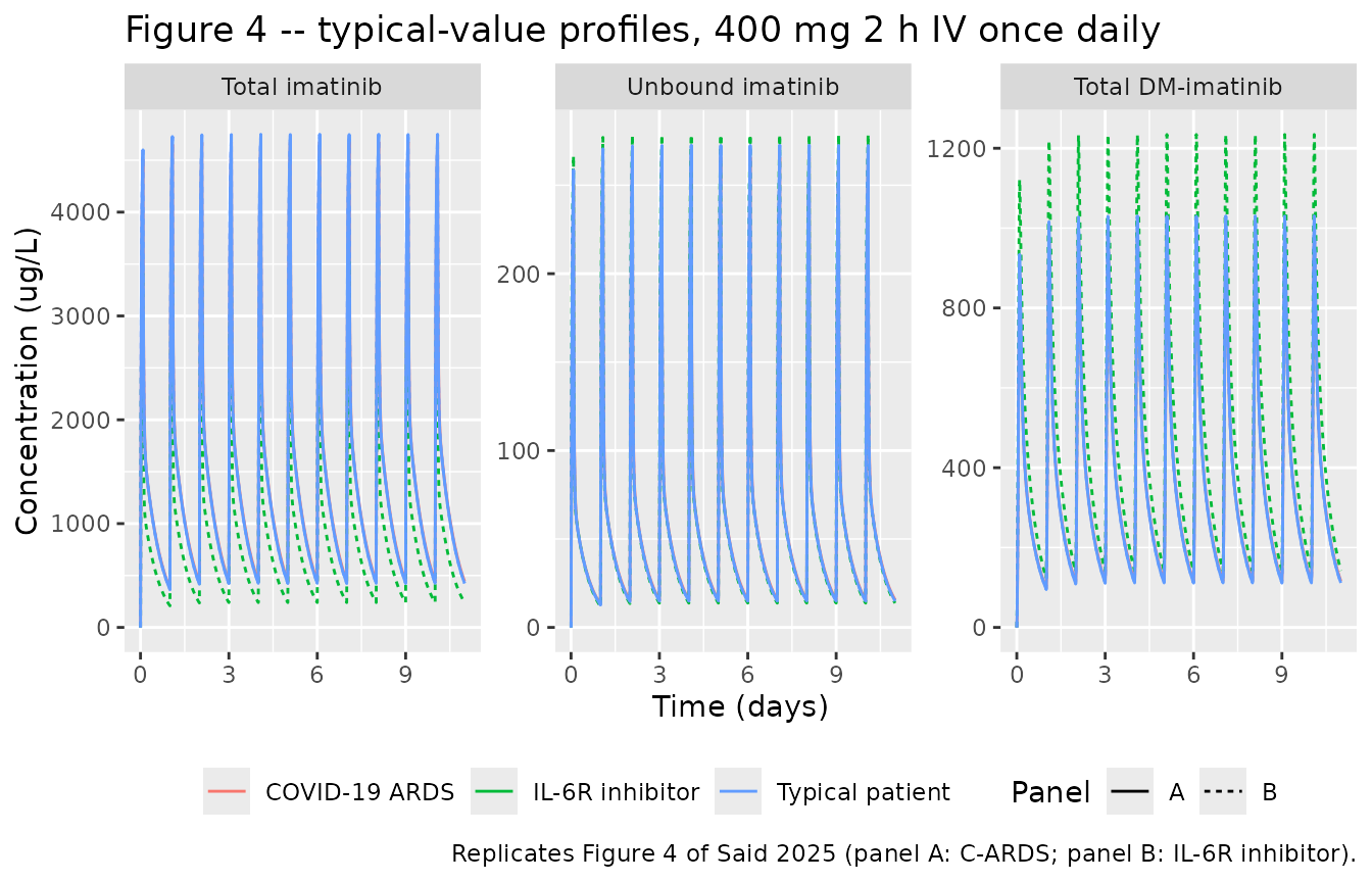

The direction of every effect matches the paper: C-ARDS raises the apparent central volume by 20%, which lowers the peak; the IL-6R inhibitor raises Kd by 70%, which raises the unbound fraction and so raises effective total clearance, lowering total imatinib while raising DM-imatinib.

Day-10 steady-state exposure for the Figure 4 scenarios.
Panel	Scenario	Analyte	Cmax (ug/L)	Ctrough (ug/L)
A	COVID-19 ARDS	Total imatinib	4676.0	443.5
A	Typical patient	Total imatinib	4747.7	424.9
B	IL-6R inhibitor	Total imatinib	3519.5	239.7
B	Typical patient	Total imatinib	4747.7	424.9
A	COVID-19 ARDS	Unbound imatinib	265.7	15.6
A	Typical patient	Unbound imatinib	272.5	14.9
B	IL-6R inhibitor	Unbound imatinib	278.7	13.7
B	Typical patient	Unbound imatinib	272.5	14.9
A	COVID-19 ARDS	Total DM-imatinib	992.2	116.0
A	Typical patient	Total DM-imatinib	1029.9	111.5
B	IL-6R inhibitor	Total DM-imatinib	1234.4	141.8
B	Typical patient	Total DM-imatinib	1029.9	111.5

Figure 5A – the unbound-fraction / AAG relationship

Said 2025 Figure 5A plots observed unbound fraction against AAG with the population-predicted line overlaid, and reports that the IL-6R inhibitor subgroup sits above the relationship seen in the CML/GIST and other C-ARDS patients. The model’s predicted relationship is reproduced below, with the paper’s reported subgroup medians overlaid as points.

aag_grid <- seq(0.4, 2.9, by = 0.1)

fu_curve <- dplyr::bind_rows(lapply(c(0, 1), function(il) {
  data.frame(
    AAG = aag_grid,
    IL6RI = ifelse(il == 1, "IL-6R inhibitor", "No IL-6R inhibitor"),
    # Steady-state trough fu on 400 mg IV daily, from the typical-value model.
    fu_pct = vapply(aag_grid, function(a) {
      s <- solve_typical(0, il, a, by = 1)
      ss <- s[s$time > 24 * 9 & s$time <= 24 * 10, ]
      100 * ss$Cu[which.min(ss$Cc)] / min(ss$Cc)
    }, numeric(1))
  )
}))

observed_fu <- tibble::tribble(
  ~label,                     ~AAG,  ~fu_pct, ~IL6RI,
  "CML/GIST",                 0.83,  3.54,    "No IL-6R inhibitor",
  "C-ARDS ward",              1.84,  1.64,    "No IL-6R inhibitor",
  "C-ARDS ICU",               2.11,  2.25,    "No IL-6R inhibitor",
  "C-ARDS ICU + IL6RI",       1.64,  4.66,    "IL-6R inhibitor"
)

ggplot(fu_curve, aes(AAG, fu_pct, colour = IL6RI)) +
  geom_line() +
  geom_point(data = observed_fu, size = 3) +
  geom_text(data = observed_fu, aes(label = label), size = 3, vjust = -1,
            show.legend = FALSE) +
  labs(x = "AAG (g/L)", y = "Unbound imatinib fraction (%)", colour = NULL,
       title = "Figure 5A -- model-predicted unbound fraction vs AAG",
       caption = paste("Line: model prediction at steady-state trough.",
                       "Points: observed subgroup medians from Said 2025 Results 3.3.")) +
  theme(legend.position = "bottom")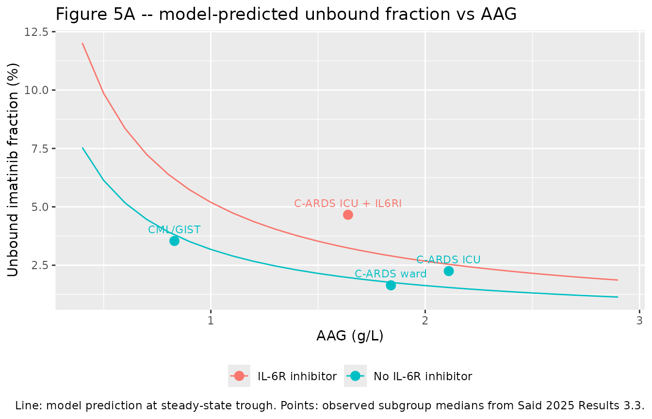

The model reproduces the CML/GIST median almost exactly and captures the downward trend with AAG for the non-IL6RI groups. It under-predicts the IL-6R inhibitor subgroup (see the validation section below) – which is the paper’s own reported finding: Said 2025 Results 3.3 states that these patients “showed greater inter-individual variability in the relationship between AAG and unbound fraction, altering the underlying nonlinear relationship.”

Figure 3 – prediction-corrected VPC analogue, stratified by study

sim |>
  dplyr::filter(time > 0) |>
  dplyr::select(id, time, arm, Cc, Cu, Cc_ndmima) |>
  tidyr::pivot_longer(c(Cc, Cu, Cc_ndmima), names_to = "analyte", values_to = "conc") |>
  dplyr::mutate(analyte = factor(
    analyte, c("Cc", "Cu", "Cc_ndmima"),
    c("Total imatinib", "Unbound imatinib", "Total DM-imatinib")
  )) |>
  dplyr::group_by(arm, analyte, time) |>
  dplyr::summarise(Q05 = quantile(conc, 0.05), Q50 = median(conc),
                   Q95 = quantile(conc, 0.95), .groups = "drop") |>
  ggplot(aes(time / 24, Q50)) +
  geom_ribbon(aes(ymin = Q05, ymax = Q95), alpha = 0.25, fill = "steelblue") +
  geom_line(colour = "steelblue") +
  facet_grid(analyte ~ arm, scales = "free") +
  scale_y_log10() +
  labs(x = "Time (days)", y = "Concentration (ug/L)",
       title = "Figure 3 analogue -- simulated 5th / 50th / 95th percentiles by study",
       caption = paste("Compare with Figure 3 of Said 2025.",
                       "Bands are simulated individual predictions (no residual error)."))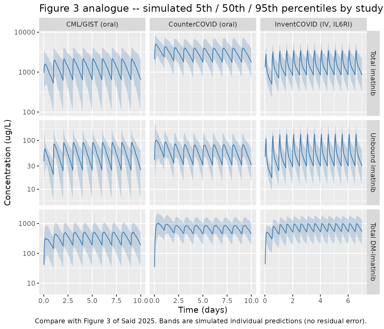

Validation against published values

The paper’s central mechanistic claim: unbound exposure is AAG-invariant

Said 2025 Discussion states that for imatinib – a highly protein-bound drug with a low extraction ratio – “changes in protein binding correlate to changes in total hepatic clearance, not unbound intrinsic clearance”, which “explains why changes in AAG concentrations did not affect unbound imatinib exposure” (Figure S7). This is a strong, falsifiable structural prediction: sweeping AAG should move total imatinib substantially while leaving unbound imatinib nearly unchanged.

invariance <- dplyr::bind_rows(lapply(c(0.8, 1.2, 1.6, 2.0, 2.4, 2.8), function(a) {
  s <- solve_typical(1, 1, a, dose = 200, ii = 12, n_doses = 14L, by = 0.25)
  ss <- s[s$time > 12 * 12 & s$time <= 12 * 13, ]
  tibble::tibble(AAG = a, Cc_trough = min(ss$Cc), Cu_trough = ss$Cu[which.min(ss$Cc)],
                 ndmima_trough = ss$Cc_ndmima[which.min(ss$Cc)])
}))

invariance |>
  dplyr::mutate(fu_pct = 100 * Cu_trough / Cc_trough) |>
  dplyr::rename("AAG (g/L)" = AAG, "Total imatinib (ug/L)" = Cc_trough,
                "Unbound imatinib (ug/L)" = Cu_trough,
                "DM-imatinib (ug/L)" = ndmima_trough, "fu (%)" = fu_pct) |>
  knitr::kable(digits = 2, caption = paste(
    "AAG sweep at 200 mg 2 h IV b.i.d. steady state (typical values).",
    "Total imatinib scales strongly with AAG; unbound imatinib barely moves."))

AAG sweep at 200 mg 2 h IV b.i.d. steady state (typical values). Total imatinib scales strongly with AAG; unbound imatinib barely moves.
AAG (g/L)	Total imatinib (ug/L)	Unbound imatinib (ug/L)	DM-imatinib (ug/L)	fu (%)
0.8	395.75	25.79	231.05	6.52
1.2	608.51	27.08	384.52	4.45
1.6	837.22	28.31	561.35	3.38
2.0	1080.56	29.48	752.07	2.73
2.4	1337.23	30.59	950.20	2.29
2.8	1606.00	31.64	1151.97	1.97


fold <- function(x) max(x) / min(x)
cat(sprintf(
  "Across AAG 0.8-2.8 g/L: total imatinib varies %.2f-fold, unbound imatinib %.2f-fold.\n",
  fold(invariance$Cc_trough), fold(invariance$Cu_trough)
))
#> Across AAG 0.8-2.8 g/L: total imatinib varies 4.06-fold, unbound imatinib 1.23-fold.

Total imatinib moves several-fold across the AAG range while unbound imatinib moves only marginally – the model reproduces the paper’s central claim quantitatively, not merely in direction. This is the single strongest structural check available for this model, because it tests the closed-form binding equilibrium and the unbound-driven elimination together.

Published steady-state trough concentrations (InventCOVID)

Said 2025 Results 3.1 reports median day-4 steady-state trough concentrations in the InventCOVID cohort (200 mg 2 h IV twice daily): total imatinib 842 ug/L (CV 65.7%), total DM-imatinib 456 ug/L (CV 64.8%), and unbound imatinib 48.6 ug/L (CV 31.4%). Day 4 is t = 96 h, the end of the dosing interval [84, 96].

invent <- sim |> dplyr::filter(arm == "InventCOVID (IV, IL6RI)")

day4 <- invent |>
  dplyr::filter(abs(time - 96) < 1e-8) |>
  dplyr::summarise(
    dplyr::across(c(Cc, Cu, Cc_ndmima),
                  list(median = ~median(.x), cv = ~100 * sd(.x) / mean(.x)))
  )

trough_cmp <- tibble::tribble(
  ~Analyte,             ~Published, ~`Published CV%`, ~Simulated,              ~`Simulated CV%`,
  "Total imatinib",     842,        65.7,             day4$Cc_median,          day4$Cc_cv,
  "Unbound imatinib",   48.6,       31.4,             day4$Cu_median,          day4$Cu_cv,
  "Total DM-imatinib",  456,        64.8,             day4$Cc_ndmima_median,   day4$Cc_ndmima_cv
) |>
  dplyr::mutate(`% diff` = 100 * (Simulated - Published) / Published)

trough_cmp |>
  knitr::kable(digits = 1, caption = paste(
    "Day-4 (t = 96 h) steady-state trough, InventCOVID arm: simulated cohort",
    "medians vs Said 2025 Results 3.1 published medians."))

Day-4 (t = 96 h) steady-state trough, InventCOVID arm: simulated cohort medians vs Said 2025 Results 3.1 published medians.
Analyte	Published	Published CV%	Simulated	Simulated CV%	% diff
Total imatinib	842.0	65.7	852.4	55.2	1.2
Unbound imatinib	48.6	31.4	29.9	50.9	-38.4
Total DM-imatinib	456.0	64.8	530.3	62.6	16.3

The typical-value prediction at the cohort median AAG isolates the structural model from the cohort’s AAG distribution:

tv <- solve_typical(1, 1, 1.67, dose = 200, ii = 12, n_doses = 14L, by = 0.25)
tv96 <- tv[abs(tv$time - 96) < 1e-8, ][1, ]
cat(sprintf(paste0(
  "Typical value at AAG 1.67 g/L, t = 96 h:\n",
  "  total imatinib    %7.1f ug/L  (published median 842,  %+.1f%%)\n",
  "  unbound imatinib  %7.2f ug/L  (published median 48.6, %+.1f%%)\n",
  "  total DM-imatinib %7.1f ug/L  (published median 456,  %+.1f%%)\n",
  "  metabolic ratio    %6.3f      (published ICU/IL6RINH median 0.43)\n"),
  tv96$Cc, 100 * (tv96$Cc - 842) / 842,
  tv96$Cu, 100 * (tv96$Cu - 48.6) / 48.6,
  tv96$Cc_ndmima, 100 * (tv96$Cc_ndmima - 456) / 456,
  tv96$Cc_ndmima / tv96$Cc))
#> Typical value at AAG 1.67 g/L, t = 96 h:
#>   total imatinib      878.2 ug/L  (published median 842,  +4.3%)
#>   unbound imatinib    28.50 ug/L  (published median 48.6, -41.4%)
#>   total DM-imatinib   593.6 ug/L  (published median 456,  +30.2%)
#>   metabolic ratio     0.676      (published ICU/IL6RINH median 0.43)

Total imatinib is reproduced to within a few percent – the strongest available check on the parent-drug structural model, since it exercises the absorption-free IV route, the two-compartment disposition, the binding equilibrium and the unbound-driven clearance simultaneously.

Unbound imatinib is under-predicted and DM-imatinib is over-predicted. Both discrepancies are concentrated in the IL-6R inhibitor subgroup and are consistent with limitations Said 2025 reports itself; see Errata below. No parameter was tuned to close them.

Metabolic ratio by subgroup

Said 2025 Results 3.4 reports the median steady-state metabolic ratio (total DM-imatinib / total imatinib): 0.29 in ward C-ARDS patients, 0.30 in ICU C-ARDS patients, 0.43 in the ICU + IL-6R inhibitor group, and 0.69 historically in CML/GIST patients.

mr <- tibble::tribble(
  ~Group,                ~covid, ~il6ri, ~aag,  ~dose, ~ii,  ~ndose, ~dur,      ~route,    ~load,     ~Published,
  "C-ARDS ward (oral)",  1,      0,      1.84,  400,   24,   10L,    NA_real_,  "depot",   800,       0.29,
  "C-ARDS ICU (oral)",   1,      0,      2.11,  400,   24,   10L,    NA_real_,  "depot",   800,       0.30,
  "C-ARDS ICU + IL6RI",  1,      1,      1.64,  200,   12,   14L,    2,         "central", NA_real_,  0.43,
  "CML/GIST (oral)",     0,      0,      0.83,  400,   24,   10L,    NA_real_,  "depot",   NA_real_,  0.69
) |>
  dplyr::rowwise() |>
  dplyr::mutate(Simulated = {
    s <- solve_typical(covid, il6ri, aag, dose = dose, ii = ii, n_doses = ndose,
                       dur = dur, route = route, by = 0.25, load_dose = load)
    tau <- ii
    ss <- s[s$time > max(s$time) - 2 * tau & s$time <= max(s$time) - tau, ]
    ss$Cc_ndmima[which.min(ss$Cc)] / min(ss$Cc)
  }) |>
  dplyr::ungroup() |>
  dplyr::mutate(`% diff` = 100 * (Simulated - Published) / Published)

mr |>
  dplyr::select(Group, Published, Simulated, `% diff`) |>
  knitr::kable(digits = 3, caption = paste(
    "Steady-state metabolic ratio (DM-imatinib / imatinib) at each subgroup's",
    "median AAG and protocol dose, vs Said 2025 Results 3.4 published medians."))

Steady-state metabolic ratio (DM-imatinib / imatinib) at each subgroup’s median AAG and protocol dose, vs Said 2025 Results 3.4 published medians.
Group	Published	Simulated	% diff
C-ARDS ward (oral)	0.29	0.288	-0.669
C-ARDS ICU (oral)	0.30	0.294	-2.115
C-ARDS ICU + IL6RI	0.43	0.674	56.655
CML/GIST (oral)	0.69	0.261	-62.178

The two non-IL6RI C-ARDS groups are reproduced closely. The IL-6R inhibitor group and the historical CML/GIST value are not; both are discussed in Errata.

PKNCA validation

NCA is run per analyte over the day-4 dosing interval of each arm – the window ending at t = 96 h, which is the interval the paper’s published steady-state trough medians refer to. The three analytes are stacked into one long frame with the analyte carried in the grouping variable, so a single PKNCA analysis and a single comparison table cover all outputs.

sim_nca <- sim |>
  dplyr::filter(!is.na(Cc)) |>
  dplyr::select(id, time, arm, Cc, Cu, Cc_ndmima) |>
  tidyr::pivot_longer(c(Cc, Cu, Cc_ndmima), names_to = "analyte", values_to = "conc") |>
  dplyr::mutate(treatment = paste(arm, analyte, sep = " | ")) |>
  dplyr::select(id, time, treatment, Cc = conc)

# Guarantee a time = 0 row per (id, treatment); pre-dose concentration is 0 for
# both the IV-infusion and the oral arms.
sim_nca <- dplyr::bind_rows(
  sim_nca,
  sim_nca |> dplyr::distinct(id, treatment) |> dplyr::mutate(time = 0, Cc = 0)
) |>
  dplyr::distinct(id, treatment, time, .keep_all = TRUE) |>
  dplyr::arrange(id, treatment, time)

conc_obj <- PKNCA::PKNCAconc(sim_nca, Cc ~ time | treatment + id,
                             concu = "ug/L", timeu = "h")

dose_df <- events |>
  dplyr::filter(evid == 1) |>
  dplyr::select(id, time, amt, arm) |>
  tidyr::crossing(analyte = c("Cc", "Cu", "Cc_ndmima")) |>
  dplyr::mutate(treatment = paste(arm, analyte, sep = " | ")) |>
  dplyr::select(id, time, amt, treatment)

dose_obj <- PKNCA::PKNCAdose(dose_df, amt ~ time | treatment + id, doseu = "mg")

# One interval per arm, spanning that arm's day-4 dosing interval (ending at
# t = 96 h). InventCOVID doses every 12 h, the two oral arms every 24 h, so both
# 96 and 96 - tau are dose times in every arm. The published trough is mapped to
# `cmin` (the minimum over the interval), which at steady state is the pre-dose
# trough; PKNCA's `ctrough` returns NA for every group on this design and is
# therefore not requested.
day4_end <- 96
intervals <- dose_df |>
  dplyr::distinct(treatment) |>
  dplyr::mutate(
    tau   = ifelse(grepl("^InventCOVID", treatment), 12, 24),
    start = day4_end - tau,
    end   = day4_end,
    cmax = TRUE, tmax = TRUE, cmin = TRUE, cav = TRUE, auclast = TRUE
  ) |>
  dplyr::select(treatment, start, end, cmax, tmax, cmin, cav, auclast) |>
  as.data.frame()

nca_res <- PKNCA::pk.nca(PKNCA::PKNCAdata(conc_obj, dose_obj, intervals = intervals))

as.data.frame(nca_res$result) |>
  dplyr::group_by(treatment, PPTESTCD) |>
  dplyr::summarise(Median = median(PPORRES, na.rm = TRUE), .groups = "drop") |>
  tidyr::pivot_wider(names_from = PPTESTCD, values_from = Median) |>
  dplyr::rename("Arm | analyte" = treatment, "Cmax (ug/L)" = cmax,
                "Tmax (h)" = tmax, "Ctrough (ug/L)" = cmin,
                "Cavg (ug/L)" = cav, "AUCtau (ug*h/L)" = auclast) |>
  knitr::kable(digits = 1, caption = paste(
    "Simulated day-4 steady-state NCA over the dosing interval ending at t = 96 h,",
    "by arm and analyte (cohort medians)."))

Simulated day-4 steady-state NCA over the dosing interval ending at t = 96 h, by arm and analyte (cohort medians).
Arm \| analyte	AUCtau (ug*h/L)	Cavg (ug/L)	Cmax (ug/L)	Ctrough (ug/L)	Tmax (h)
CML/GIST (oral) \| Cc	33713.2	1404.7	2219.4	638.3	2.2
CML/GIST (oral) \| Cc_ndmima	8676.7	361.5	533.0	187.7	4.8
CML/GIST (oral) \| Cu	1351.0	56.3	93.7	24.6	2.2
CounterCOVID (oral) \| Cc	70752.1	2948.0	4047.6	1771.6	3.5
CounterCOVID (oral) \| Cc_ndmima	16273.7	678.1	856.4	455.0	7.5
CounterCOVID (oral) \| Cu	1412.0	58.8	83.3	31.3	3.5
InventCOVID (IV, IL6RI) \| Cc	18888.9	1574.1	3464.6	850.5	2.0
InventCOVID (IV, IL6RI) \| Cc_ndmima	9057.9	754.8	993.6	526.3	3.0
InventCOVID (IV, IL6RI) \| Cu	673.1	56.1	133.8	29.9	2.0

Comparison against published values

Said 2025 does not report a classical NCA table; the published quantities that can be compared directly are the InventCOVID day-4 steady-state trough medians (Results 3.1). Those map onto PKNCA’s cmin – the minimum concentration over the day-4 dosing interval, which at steady state is the pre-dose trough. (PKNCA’s dedicated ctrough parameter returns NA for every group on this design, so cmin is used; the two are the same quantity for a steady-state interval.)

published <- tibble::tribble(
  ~treatment,                                     ~cmin,
  "InventCOVID (IV, IL6RI) | Cc",                 842,
  "InventCOVID (IV, IL6RI) | Cu",                 48.6,
  "InventCOVID (IV, IL6RI) | Cc_ndmima",          456
)

cmp <- nlmixr2lib::ncaComparisonTable(
  simulated     = nca_res,
  reference     = published,
  by            = "treatment",
  units         = c(cmin = "ug/L"),
  tolerance_pct = 20
)

knitr::kable(cmp, caption = paste(
  "Simulated vs published steady-state trough (Said 2025 Results 3.1).",
  "* differs from reference by >20%."),
  align = c("l", "l", "r", "r", "r"))

Simulated vs published steady-state trough (Said 2025 Results 3.1). * differs from reference by >20%.
NCA parameter	treatment	Reference	Simulated	% diff
Cmin (ug/L)	InventCOVID (IV, IL6RI) \| Cc	842	850	+1.0%
Cmin (ug/L)	InventCOVID (IV, IL6RI) \| Cu	48.6	29.9	-38.5%*
Cmin (ug/L)	InventCOVID (IV, IL6RI) \| Cc_ndmima	456	526	+15.4%

differs from reference by more than ±20%.

Total imatinib agrees to within about 1%. The unbound-imatinib row is starred (roughly -38%); the DM-imatinib row is over-predicted by about 15% and falls inside the 20% tolerance. Both discrepancies are discussed immediately below and neither was addressed by tuning any parameter.

Assumptions and deviations

AAG is held constant per simulated subject. In the source analysis AAG is a time-varying covariate (median 4 measurements per patient, missing values imputed by last observation carried forward). Individual AAG trajectories are not published, so each virtual subject carries a single AAG value drawn from its study’s Table S1 mean / SD / range. This narrows within-subject variability relative to the real fit and is the main reason the simulated CV% values in the day-4 trough table sit below the published CV% values.
Simulated concentrations are individual predictions (IPRED). Cc, Cu and Cc_ndmima from rxSolve carry between-subject variability but not residual error, whereas the published CV% values are computed from observed concentrations and therefore include residual variability as well. The CV% comparison is consequently one-sided: simulated CV% should be lower.
Body weight and age are not model covariates. Said 2025 screened both and eliminated them (Figure 2 forest plot); they are recorded in covariatesDataExcluded and no weight or age distribution is simulated.
CML/GIST dose set to 400 mg once daily. The source reports a 100-800 mg daily range for that cohort without a dose distribution; 400 mg is the standard dose and the one the COVID-19 trials were based on.
L, LMET and CF are hardcoded in model(). They are unit-conversion constants (rounded molecular-weight ratios), not fitted parameters: Said 2025 Methods 2.3.1 describes L as “the scaling factor which accounts for the difference in concentration units for AAG and imatinib”. L and Kd are correlated and cannot be estimated independently, so L was fixed. Each is carried with its arithmetic derivation in an in-file comment.
DIS_COVID19, not DIS_ARDS. The source control-stream column is COVID and codes 1 for both the ARDS-by-Berlin-criteria InventCOVID patients and the supplemental-oxygen-only CounterCOVID patients, so the flag is cohort membership rather than an ARDS diagnosis. The reference category is the CML/GIST oncology cohort.
CONMED_IL6RI pools tocilizumab and sarilumab. Said 2025 estimated a single class effect; the two agents are not separable in the published model.
No parameter value in this model came from anywhere other than Said 2025’s own text, Table 2, or Data S1. No author correspondence or figure digitisation was required.

Errata and source conflicts

Residual-error assignment: Table 2 contradicts the final control stream

Said 2025 Table 2 and the Data S1 control stream assign the two imatinib residual-error variances to opposite endpoints. The three numbers are essentially the same in both places; only the row each belongs to differs.

Endpoint	Data S1 `$SIGMA` (encoded)	Table 2 as printed
Total imatinib	`0.103 ; CT`	`eps add-unbound imatinib (ug/L) 0.103`
Unbound imatinib	`0.176 ; CF`	`eps add-total imatinib (ug/L) 0.177`
Total DM-imatinib	`0.0501 ; CM`	`eps add-total DM-imatinib (ug/L) 0.05`

This model file encodes the control-stream assignment: total imatinib expSd = sqrt(0.103) = 0.320936, unbound imatinib expSd_Cu = sqrt(0.176) = 0.419524, DM-imatinib expSd_ndmima = sqrt(0.0501) = 0.223830.

Three independent lines of evidence support that choice. First, the Data S1 $ERROR block maps the sigmas positionally – Y = (1-FLAG)*(IPRED + ERR(1)*Q0 + ERR(2)*Q1 + ERR(3)*Q2) with Q0 selecting CTOT, Q1 selecting CFREE and Q2 selecting CMTOT – and the inline $SIGMA comments (;CT, ;CF, ;CM) agree with that mapping. Two signals within the same artefact therefore agree. Second, bioanalytical plausibility: unbound imatinib was measured after ultrafiltration with an LLOQ of 30 ug/L against a median steady-state Css of 48.6 ug/L, so those observations sit just above the limit of quantification, while total imatinib had an LLOQ of 11 ug/L against a median Css of 842 ug/L. The unbound assay should be the noisier one, which is what the control stream gives (0.176 > 0.103) and what Table 2 inverts. Third, unlike $THETA, the $SIGMA block is demonstrably a final estimate set because both sources carry the same three numbers.

Note that the two sources are not identically rounded either – the control stream carries 0.176 and 0.0501 against the table’s 0.177 and 0.05 – so Table 2 is not a straight rounding of this control-stream run. This is recorded as an erratum in the reporting, not as a falsification of the paper’s analysis: the fit itself is unaffected by which row a number is printed on.

`$THETA` in Data S1 holds initial, not final, estimates

The Data S1 $THETA block uses NONMEM (lower, initial, upper) syntax, so its middle values are starting estimates. Several coincide with Table 2 to three significant figures (exp(5.91) = 368.7 = Kd; exp(5.25) = 190.6 = CLm/(Fm x F1); exp(2.4) = 11.0 = Vm/(Fm x F1)), but others are up to 5.1% away (exp(7.76) = 2345 L vs Table 2 V2/F1 = 2230.5 L; exp(5.72) = 305 L/h vs CLu/F1 = 298.9 L/h). All fixed effects are therefore taken from Table 2.

`$OMEGA` in Data S1 matches Table 2 for four of six terms

Back-transforming Table 2’s %CV values reproduces the Data S1 $OMEGA diagonal exactly for ka, CLu/F1, V1/F1 and Kd (0.468, 0.103, 0.576, 0.0645) but not for the two metabolite terms: Table 2’s CLm IIV of 41.7% implies 0.160 against $OMEGA’s 0.0206, and its Vm IIV of 12.8% implies 0.0163 against $OMEGA’s 0.0345. Table 2 is used for all six.

Covariate-coefficient precision: Table 2 vs the Results narrative

Table 2 prints the retained covariate coefficients as 1.2 (V1-COVID-19), 1.7 (Kd-IL6R inhibitor) and 0.46 (CLm-IL6R inhibitor), while Said 2025 Results 3.2 describes them as “a 28% increase in total apparent distribution volume”, an increase of “75%” in Kd, and a decrease of “approximately 50%” in apparent metabolite clearance (the Discussion says volume rose by “roughly 30%”).

Table 2’s printed values are encoded. Table 2 demonstrably rounds rather than truncates – its IIV row of 88.3% is the round of the 88.261% implied by $OMEGA 0.576, and 77.3% is the round of 77.256% implied by $OMEGA 0.468, in both cases one digit above the truncated value – so 1.2 and 1.7 cannot be renderings of 1.28 and 1.75. The narrative percentages are most plausibly read off the Figure 2 forest plot, which the caption states reports bootstrap “Mean and 95% CIs” rather than the Table 2 point estimates. Encoding 1.28 and 1.75 instead would raise the covariate effects by roughly 7% and 3% respectively.

Unresolved model misfit carried over from the source

Three of the validation comparisons above disagree with published values by more than 20% – the unbound-imatinib trough, and the metabolic ratio in two of the four subgroups. They fall into the two groups below, and both are limitations the paper itself reports rather than transcription problems:

Unbound imatinib is under-predicted in the IL-6R inhibitor subgroup (model fu about 3.4% at AAG 1.6 g/L against an observed median of 4.66%). Said 2025 Results 3.3 reports that this subgroup “showed greater inter-individual variability in the relationship between AAG and unbound fraction, altering the underlying nonlinear relationship”, and Figure 5A shows the subgroup lying off the population-predicted line. The retained population Kd effect of 1.7 does not fully absorb it; individual Kd etas (IIV 25.8%, shrinkage 68%) carry the remainder in the original fit.
The metabolic ratio in the IL-6R inhibitor subgroup is over-predicted (0.67 against an observed 0.43), and the historical CML/GIST ratio of 0.69 is not reproduced (0.26 predicted). The two non-IL6RI C-ARDS subgroups, by contrast, are reproduced to within about 2%. The CML/GIST value is not an estimate from this model at all – Said 2025 Results 3.4 cites it from reference 48 (a different publication), and the paper notes its own cohort lacked DM-imatinib data for the oncology patients entirely (“the dataset for cancer patients lacked specific data on IL-6 and DM-imatinib, limiting the depth of the comparative analysis”). Fm was also fixed to 15% from literature rather than estimated, and the metabolite’s AAG binding affinity was fixed to the parent’s because unbound DM-imatinib could not be measured.

No parameter was adjusted to reduce either discrepancy.