Clozapine and norclozapine (Olmos 2019) • nlmixr2lib

Model and source

Citation: Olmos I, Ibarra M, Vazquez M, Maldonado C, Fagiolino P, Giachetto G (2019). Population Pharmacokinetics of Clozapine and Norclozapine and Switchability Assessment between Brands in Uruguayan Patients with Schizophrenia. BioMed Research International 2019:3163502. doi:10.1155/2019/3163502.
Description: Simultaneous one-compartment parent-plus-metabolite population PK model for oral clozapine (CZP) and its active metabolite norclozapine (NCZP) in 98 Uruguayan adult inpatients (76 male, 22 female) with DSM-IV schizophrenia, fit to 171 steady-state morning trough observations per analyte (Olmos 2019). First-order absorption (ka fixed at 1.24 1/h from Jerling 1996) into a clozapine central compartment with first-order elimination; complete (f = 1) conversion of clozapine to norclozapine is assumed, so the whole clozapine elimination flux feeds a second one-compartment metabolite compartment after a molecular-weight correction. Both apparent volumes of distribution are fixed from Golden and Honigfeld (750 L clozapine, 1860 L norclozapine at 70 kg) and scale linearly with body weight; both apparent clearances scale with body weight to the fixed allometric 0.75 power. Smoking status was the only covariate retained in the final model: clozapine apparent clearance is estimated separately in nonsmokers (28.1 L/h) and smokers (36.5 L/h). The study switched patients from the brand-name product (Leponex) to a similar product (Luverina), so a relative bioavailability of 0.892 for Luverina versus the Leponex reference (whose F is the fixed 1 anchor) is estimated together with its own between-subject variability. Clozapine and norclozapine apparent clearances carry correlated between-subject variability; residual error is proportional and separate per analyte.
Article: https://doi.org/10.1155/2019/3163502 (BioMed Research International 2019:3163502, PMC6431368; open access under CC BY).
Supplement: none. The publisher deposit for this article contains only the three figure files; there is no supplementary text, parameter table or NONMEM control stream.
Errata: none. CrossRef reports no update-to / updated-by relation for this DOI and Europe PMC returns no citing correction notice.

Population

Olmos 2019 studied 98 adult inpatients (76 male, 22 female) of Hospital Vilardebo in Montevideo, Uruguay, with a DSM-IV diagnosis of schizophrenia. The cohort had a median age of 39 years (range 20-68), a median body weight of 78 kg (48-137) and a median BMI of 26 kg/m^2 (15-43); the final dataset describes the patients as Caucasian (Table 1).

Every patient had been treated with brand-name clozapine (Leponex, Novartis) for more than one year when the hospital’s purchasing switched to the “similar” product (Luverina, Celsius). Patients were on Luverina for two months before the second blood sample, so the design is a sequential switch rather than a randomised crossover. Oral clozapine was given twice daily at a median 350 mg/day (range 150-700), and 68 of the 73 patients who completed both periods (93%) kept the same regimen across the switch.

The data are very sparse: a single morning predose (trough) sample per subject per period, taken at steady state under unchanged comedication. 171 trough observations were recorded for each analyte, of which 146 came from the 73 patients who completed both periods; 25 patients contributed one period only (17 Luverina, 8 Leponex). Because only one observation per subject per period was available, interoccasion variability was not identifiable and Cmax,ss / Tmax,ss could not be estimated – limitations the authors state explicitly.

Concentrations were measured by HPLC-UV at 230 nm with medazepam as internal standard, linear over 54.8-1086 ng/mL (clozapine) and 72.3-1085 ng/mL (norclozapine). All clozapine observations were above the LLOQ; left-censored norclozapine values were under 4% of the total and were included as observed.

The same information is available programmatically from the model’s population metadata:

str(ui$population, max.level = 1)
#> List of 16
#>  $ species       : chr "human"
#>  $ n_subjects    : int 98
#>  $ n_observations: int 171
#>  $ n_studies     : int 1
#>  $ age_range     : chr "20-68 years (median 39; Table 1)"
#>  $ age_median    : chr "39 years"
#>  $ weight_range  : chr "48-137 kg (median 78; Table 1)"
#>  $ weight_median : chr "78 kg"
#>  $ bmi_range     : chr "15-43 kg/m^2 (median 26; Table 1)"
#>  $ sex_female_pct: num 22.4
#>  $ race_ethnicity: Named num 100
#>   ..- attr(*, "names")= chr "White"
#>  $ disease_state : chr "DSM-IV-diagnosed schizophrenia, inpatients of Hospital Vilardebo, Montevideo, Uruguay. All patients had been tr"| __truncated__
#>  $ dose_range    : chr "Oral clozapine 150-700 mg/day (median 350 mg/day; Table 1), administered twice a day with each brand. 68 of the"| __truncated__
#>  $ smoke_strata  : chr "46 smokers (37 male), 52 nonsmokers (39 male) (Table 1)"
#>  $ regions       : chr "Uruguay (single centre, Hospital Vilardebo, Montevideo)"
#>  $ notes         : chr "Very sparse therapeutic-drug-monitoring design: a single morning predose (trough) sample per subject per treatm"| __truncated__

Source trace

The per-parameter origin is recorded as an in-file comment next to each ini() entry in inst/modeldb/specificDrugs/Olmos_2019_clozapine.R. The table below collects them in one place.

Equation / parameter	Value	Source location
`lka`	`log(1.24)`, fixed	Methods 2.3: “ka was fixed to a value of 1.24 h-1 as estimated by Jerling et al. [31]”
`lcl_nonsmoke`	`log(28.1)`	Table 2, “CLap CZP (L/h)” / “Clozapine apparent elimination clearance in nonsmokers”, 28.1 (RSE 6%)
`lcl_smoke`	`log(36.5)`	Table 2, “CLap CZP SMK (L/h)” / “Clozapine apparent elimination clearance in smokers”, 36.5 (RSE 8%)
`lcl_norcloz`	`log(53.6)`	Table 2, row 3 / “Norclozapine apparent elimination clearance”, 53.6 (RSE 6%)
`lvc`	`log(750)`, fixed	Methods 2.3, apparent V/F of clozapine at 70 kg, from Golden and Honigfeld [30]
`lvc_norcloz`	`log(1860)`, fixed	Methods 2.3, apparent V/F of norclozapine at 70 kg, from Golden and Honigfeld [30]
`e_wt_cl`, `e_wt_cl_norcloz`	`0.75`, fixed	Methods Eq. (2), `CLapi = CLap * (BWi/70)^0.75`, “fixing this value to the allometric standard of 0.75”
`e_wt_vc`, `e_wt_vc_norcloz`	`1`, fixed	Methods Eq. (1), `Vi = V * (BWi/70)`, “a proportional centered model”
`lfdepot_leponex`	`log(1)`, fixed	Methods 2.3: “F was fixed to 1 for Leponex”
`lfdepot_luverina`	`log(0.892)`	Table 2, “F Luverina” / relative bioavailability of Luverina vs Leponex, 0.892 (RSE 6%)
`etalcl`	`0.171841`	Table 2, “BSV CLap CZP (%)” = 43.3; `omega^2 = log(1 + 0.433^2)`
`etalcl_norcloz`	`0.222344`	Table 2, “BSV CLap NCZP (%)” = 49.9; `omega^2 = log(1 + 0.499^2)`
covariance `etalcl:etalcl_norcloz`	`0.108876`	Table 2, “cov CLap CZP - CLap NCZP (%)” = 55.7, read as correlation 0.557 (see Errata)
`etalfdepot_luverina`	`0.174034`	Table 2, “BSV F (%)” = 43.6; `omega^2 = log(1 + 0.436^2)`
`propSd`	`0.0954`	Table 2, “Proportional clozapine (%)” = 9.54 (RSE 21%)
`propSd_norcloz`	`0.153`	Table 2, “Proportional norclozapine (%)” = 15.3 (RSE 15%)
`d/dt(depot)`, `d/dt(central)`	n/a	Methods 2.3, “a one-compartment disposition for both substances” with first-order absorption
`d/dt(central_norcloz)`	n/a	Methods 2.3, “Complete conversion of CZP into NCZP was assumed and a factor was included in NCZP formation to account for the molecular weight differences”
`mw_cloz / mw_norcloz`	`326.83` / `312.80` g/mol	Not from the paper. Compound formulae C18H19ClN4 / C17H17ClN4; see Errata
`Cc ~ prop(propSd)`	n/a	Methods Eq. (4), `Cik = Cpred * (1 + eps_ik)`

Structural checks against closed forms

Before any cohort is simulated, the packaged model is checked against the arithmetic the paper’s own equations imply. These are deterministic identities, so they are gated tightly.

mod <- readModelDb("Olmos_2019_clozapine")
mod_typical <- rxode2::zeroRe(mod)

# Molecular-weight factor the paper describes but does not print.
mw_ratio <- 312.80 / 326.83

# Five typical-value scenarios that each isolate one structural feature.
scenarios <- tibble::tribble(
  ~id, ~scenario,            ~WT, ~SMOKE, ~FORM_CZP_LUVERINA, ~daily_mg,
  1L,  "reference",           70,      0,                  0,       400,
  2L,  "smoker",              70,      1,                  0,       400,
  3L,  "Luverina",            70,      0,                  1,       400,
  4L,  "140 kg",             140,      0,                  0,       400,
  5L,  "smoker + Luverina",   70,      1,                  1,       400
)

# 60 days of twice-daily dosing loads both analytes to steady state, then one
# fully-resolved dosing interval is observed. The typical norclozapine half-life
# is only ~24.7 h at 70 kg, but the between-subject variability on its apparent
# clearance (CV 49.9%) puts the slowest subjects near 100 h, and at 21 days
# those subjects are still ~1.4% short of steady state -- enough to break the
# cohort mass balance below (measured: max |residual| 1.4e-2 at 42 doses,
# 7.9e-5 at 90, 8.0e-5 at 140, i.e. the trapezoid floor is reached by 90).
tau <- 12
n_dose <- 120L
t_last <- tau * (n_dose - 1L)
grid <- c(0, seq(0.1, 4, by = 0.1), seq(4.5, tau, by = 0.5))

# Observations are written on the ODE state `central`, never on the algebraic
# observable `Cc` -- referencing an observable as a compartment auto-injects a
# `cmt()` slot after the ODE states and renumbers them. Because the model
# carries two endpoints (`Cc` and `Cc_norcloz`), each observation row also needs
# a `dvid`; rxode2 still returns BOTH observables as columns on every row.
make_events <- function(subj, tau = 12, n_dose = 42L, grid) {
  t_last <- tau * (n_dose - 1L)
  doses <- subj |>
    tidyr::crossing(time = seq(0, t_last, by = tau)) |>
    dplyr::mutate(
      evid = 1L, amt = daily_mg / (24 / tau), cmt = "depot",
      dvid = NA_integer_
    )
  obs <- subj |>
    tidyr::crossing(time = t_last + grid) |>
    dplyr::mutate(evid = 0L, amt = NA_real_, cmt = "central", dvid = 1L)
  dplyr::bind_rows(doses, obs) |>
    dplyr::arrange(id, time, evid)
}

ev_typ <- make_events(scenarios, tau = tau, n_dose = n_dose, grid = grid)
stopifnot(!anyDuplicated(unique(ev_typ[, c("id", "time", "evid")])))

sim_typ <- rxode2::rxSolve(
  mod_typical,
  events = ev_typ,
  keep = c("scenario", "daily_mg"),
  useLinCmt = FALSE
) |>
  as.data.frame() |>
  # rxSolve returns observation records only (addDosing defaults to FALSE).
  dplyr::mutate(tad = time - t_last)
#> ℹ omega/sigma items treated as zero: 'etalcl', 'etalcl_norcloz', 'etalfdepot_luverina'
#> Warning: multi-subject simulation without without 'omega'

# The explicit metabolite ODE must have been solved: if rxode2 had silently
# auto-solved a linCmt() parent model it would be absent from the output.
stopifnot(all(c("Cc", "Cc_norcloz", "central_norcloz", "cl", "frel") %in% names(sim_typ)))

# Interval summaries per scenario, using a linear-up / log-down trapezoid on
# the 0.1 h grid through Tmax (~2.5 h).
trap <- function(t, y) sum(diff(t) * (head(y, -1) + tail(y, -1)) / 2)

interval <- sim_typ |>
  dplyr::group_by(id, scenario, daily_mg) |>
  dplyr::summarise(
    cl = dplyr::first(cl),
    cl_norcloz = dplyr::first(cl_norcloz),
    frel = dplyr::first(frel),
    auc_czp = trap(tad, Cc),
    auc_ncz = trap(tad, Cc_norcloz),
    ctrough_czp = Cc[which.max(tad)],
    ctrough_ncz = Cc_norcloz[which.max(tad)],
    c0_czp = Cc[which.min(tad)],
    .groups = "drop"
  ) |>
  dplyr::mutate(dose_interval = daily_mg / (24 / tau))

# (a) Steady state has been reached: the concentration at the start of the
#     observed interval equals the concentration at its end.
ss_gap <- with(interval, max(abs(ctrough_czp / c0_czp - 1)))

# (b) Clozapine mass balance over one steady-state interval:
#     CL/F * AUCtau == F_rel * dose. Cc is ng/mL, so divide by 1000 for mg/L.
mb_czp <- with(interval, cl * auc_czp / 1000 / (frel * dose_interval) - 1)

# (c) Norclozapine mass balance: the whole clozapine elimination flux becomes
#     norclozapine after the molecular-weight correction.
mb_ncz <- with(interval, cl_norcloz * auc_ncz / 1000 /
  (mw_ratio * frel * dose_interval) - 1)

pick <- function(what, sc) interval[[what]][match(sc, interval$scenario)]

gates <- tibble::tibble(
  Check = c(
    "Steady state reached (Cc at interval start == at interval end)",
    "Clozapine CL/F * AUCtau == F * dose",
    "Norclozapine CL/F * AUCtau == (MWncz/MWczp) * F * dose",
    "Smoking: AUC(smoker)/AUC(nonsmoker) for clozapine == 28.1/36.5",
    "Smoking has no effect on norclozapine AUC (ratio == 1)",
    "Luverina: AUC ratio vs Leponex == 0.892 (clozapine)",
    "Luverina: AUC ratio vs Leponex == 0.892 (norclozapine)",
    "Allometry: AUC(140 kg)/AUC(70 kg) == (70/140)^0.75"
  ),
  Expected = c(
    0, 0, 0,
    28.1 / 36.5, 1, 0.892, 0.892, (70 / 140)^0.75
  ),
  Achieved = c(
    ss_gap,
    max(abs(mb_czp)),
    max(abs(mb_ncz)),
    pick("auc_czp", "smoker") / pick("auc_czp", "reference"),
    pick("auc_ncz", "smoker") / pick("auc_ncz", "reference"),
    pick("auc_czp", "Luverina") / pick("auc_czp", "reference"),
    pick("auc_ncz", "Luverina") / pick("auc_ncz", "reference"),
    pick("auc_czp", "140 kg") / pick("auc_czp", "reference")
  )
) |>
  dplyr::mutate(`Abs. difference` = abs(Achieved - Expected))

knitr::kable(gates, digits = 6, caption = "Deterministic structural checks.")

Deterministic structural checks.
Check	Expected	Achieved	Abs. difference
Steady state reached (Cc at interval start == at interval end)	0.000000	0.000000	0.0e+00
Clozapine CL/F * AUCtau == F * dose	0.000000	0.000030	3.0e-05
Norclozapine CL/F * AUCtau == (MWncz/MWczp) * F * dose	0.000000	0.000017	1.7e-05
Smoking: AUC(smoker)/AUC(nonsmoker) for clozapine == 28.1/36.5	0.769863	0.769862	1.0e-06
Smoking has no effect on norclozapine AUC (ratio == 1)	1.000000	0.999996	4.0e-06
Luverina: AUC ratio vs Leponex == 0.892 (clozapine)	0.892000	0.892000	0.0e+00
Luverina: AUC ratio vs Leponex == 0.892 (norclozapine)	0.892000	0.892000	0.0e+00
Allometry: AUC(140 kg)/AUC(70 kg) == (70/140)^0.75	0.594604	0.594605	1.0e-06


# Tolerances, tightest first, each set by what the identity actually is rather
# than by what one run happened to give:
#   rows 6-7 (Luverina) rescale the whole profile by a constant, so numerator
#     and denominator carry the identical trapezoid error and it cancels
#     exactly -- realised 0 to machine precision.
#   rows 4, 5, 8 (smoking, allometry) change the profile SHAPE, so the two
#     trapezoid errors no longer cancel -- realised 1.4e-6, 2.7e-6, 1.2e-6 on
#     this 0.1 h grid.
#   rows 2-3 are the absolute trapezoid error of AUCtau -- realised 3.0e-5.
#   row 1 is the steady-state residual after 60 days -- realised below the
#     6-digit print resolution (5.8e-8 at the 42-dose loading originally tried).
stopifnot(
  gates$`Abs. difference`[1] < 1e-5,
  all(gates$`Abs. difference`[2:3] < 1e-3),
  all(gates$`Abs. difference`[c(4, 5, 8)] < 1e-4),
  all(gates$`Abs. difference`[6:7] < 1e-9)
)

The mass-balance gates above are only meaningful if they can fail. The control below perturbs the clearance by 10% and confirms the clozapine gate goes red:

mb_mutated <- with(interval, (1.1 * cl) * auc_czp / 1000 / (frel * dose_interval) - 1)
stopifnot(max(abs(mb_mutated)) > 0.05)
cat("mutation control: 10% clearance perturbation moves the mass-balance",
  "residual to", sprintf("%.4f", max(abs(mb_mutated))), "(gate threshold 1e-3)\n")
#> mutation control: 10% clearance perturbation moves the mass-balance residual to 0.1000 (gate threshold 1e-3)

Steady-state profiles

Olmos 2019 publishes no concentration-time figure – its Figure 1 is an NPC coverage plot, Figure 2 an NPDE plot and Figure 3 an in vitro dissolution profile, none of which is a simulation output of the PK model. The panel below is therefore a model prediction rather than a replication of a published figure, shown so the structure the trough data constrain is visible.

sim_typ |>
  dplyr::filter(scenario %in% c("reference", "smoker")) |>
  dplyr::select(tad, scenario, Clozapine = Cc, Norclozapine = Cc_norcloz) |>
  tidyr::pivot_longer(c(Clozapine, Norclozapine),
    names_to = "Analyte", values_to = "conc"
  ) |>
  ggplot(aes(tad, conc, colour = scenario, linetype = Analyte)) +
  geom_line(linewidth = 0.8) +
  labs(
    x = "Time after dose (h)", y = "Concentration (ng/mL)",
    colour = "Smoking status", linetype = NULL,
    title = "Predicted steady-state interval, 70 kg, 200 mg twice daily (Leponex)",
    caption = "Model prediction; Olmos 2019 publishes no concentration-time figure."
  ) +
  theme_bw()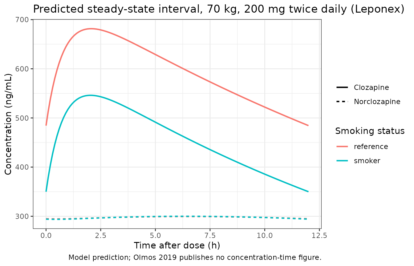

Virtual cohort

Individual data are not public, so two virtual cohorts are built whose body weights and daily doses follow the per-stratum medians and ranges of Table 1. Table 1 stratifies the same 171 records two different ways – by smoking status and by brand – and the two stratifications have different weight and dose distributions, so each is reproduced with its own cohort rather than by slicing a single pooled one.

# `set.seed()` seeds R's RNG, which is what draws the covariates below. It does
# NOT seed rxode2's simulation RNG, and rxode2's streams are partitioned per
# solver thread -- so the eta draws differ between a 2-core CI runner and a
# 16-thread workstation. Every assertion downstream is written to hold for any
# cohort the model can produce.
set.seed(20190306)

# Truncated-lognormal draw matching a published median and min-max range. The
# log-scale SD is set so the observed range spans roughly +/- 2.6 SD, which is
# the expected extreme spread for n ~ 100.
draw_lognorm <- function(n, med, lo, hi, digits = 1) {
  sdlog <- mean(abs(c(log(hi / med), log(lo / med)))) / 2.6
  round(pmin(pmax(stats::rlnorm(n, log(med), sdlog), lo), hi), digits)
}

# Daily clozapine doses are prescribed in 25 mg steps.
draw_dose <- function(n, med, lo, hi) {
  pmin(pmax(round(draw_lognorm(n, med, lo, hi, digits = 3) / 25) * 25, lo), hi)
}

make_cohort <- function(n, stratum, wt_med, wt_lo, wt_hi,
                        dose_med, dose_lo, dose_hi,
                        smoke_p, luverina_p, id_offset = 0L) {
  tibble::tibble(
    id = id_offset + seq_len(n),
    stratum = stratum,
    WT = draw_lognorm(n, wt_med, wt_lo, wt_hi),
    daily_mg = draw_dose(n, dose_med, dose_lo, dose_hi),
    SMOKE = if (is.na(smoke_p)) {
      NA_integer_
    } else {
      stats::rbinom(n, 1L, smoke_p)
    },
    FORM_CZP_LUVERINA = if (is.na(luverina_p)) {
      NA_integer_
    } else {
      stats::rbinom(n, 1L, luverina_p)
    }
  )
}

# Cohort A -- the smoking stratification (Table 1 columns "Smoking" and
# "Nonsmoking"). Sizes are 3x the published stratum sizes (46 / 52), which keeps
# the published 46:52 balance and stays inside the 200-per-arm cap. The brand
# mix within each arm follows the 81:90 record split.
cohort_a <- dplyr::bind_rows(
  make_cohort(138L, "Smoking", 78, 48, 120, 350, 150, 700,
    smoke_p = NA, luverina_p = 90 / 171, id_offset = 0L
  ) |> dplyr::mutate(SMOKE = 1L),
  make_cohort(156L, "Nonsmoking", 80, 57, 137, 400, 200, 650,
    smoke_p = NA, luverina_p = 90 / 171, id_offset = 1000L
  ) |> dplyr::mutate(SMOKE = 0L)
)

# Cohort B -- the brand stratification (Table 1 columns "Leponex" and
# "Luverina"). Sizes are 2x the published record counts (81 / 90).
cohort_b <- dplyr::bind_rows(
  make_cohort(162L, "Leponex", 77, 48, 136, 400, 200, 600,
    smoke_p = 46 / 98, luverina_p = NA, id_offset = 2000L
  ) |> dplyr::mutate(FORM_CZP_LUVERINA = 0L),
  make_cohort(180L, "Luverina", 82, 54, 137, 350, 150, 700,
    smoke_p = 46 / 98, luverina_p = NA, id_offset = 3000L
  ) |> dplyr::mutate(FORM_CZP_LUVERINA = 1L)
)

subjects <- dplyr::bind_rows(
  cohort_a |> dplyr::mutate(cohort = "smoking"),
  cohort_b |> dplyr::mutate(cohort = "brand")
)

events <- make_events(subjects, tau = tau, n_dose = n_dose, grid = grid)
stopifnot(
  !anyDuplicated(unique(events[, c("id", "time", "evid")])),
  nrow(dplyr::distinct(subjects, id)) == nrow(subjects)
)

subjects |>
  dplyr::group_by(stratum) |>
  dplyr::summarise(
    N = dplyr::n(),
    `Weight median (kg)` = stats::median(WT),
    `Weight range (kg)` = sprintf("%.0f-%.0f", min(WT), max(WT)),
    `Dose median (mg/day)` = stats::median(daily_mg),
    `Dose range (mg/day)` = sprintf("%.0f-%.0f", min(daily_mg), max(daily_mg)),
    `Smokers (%)` = round(100 * mean(SMOKE)),
    .groups = "drop"
  ) |>
  knitr::kable(caption = "Simulated cohort characteristics; compare with Table 1 of Olmos 2019.")

Simulated cohort characteristics; compare with Table 1 of Olmos 2019.
stratum	N	Weight median (kg)	Weight range (kg)	Dose median (mg/day)	Dose range (mg/day)	Smokers (%)
Leponex	162	80.90	48-136	400	200-600	48
Luverina	180	82.95	54-134	350	175-700	48
Nonsmoking	156	80.30	57-137	400	200-650	0
Smoking	138	77.45	53-120	350	175-700	100

Simulation

sim <- rxode2::rxSolve(
  mod,
  events = events,
  keep = c("stratum", "cohort", "daily_mg"),
  useLinCmt = FALSE
) |>
  as.data.frame() |>
  # rxSolve returns observation records only (addDosing defaults to FALSE).
  dplyr::mutate(tad = time - t_last)

stopifnot(
  nrow(sim) > 0,
  all(c("Cc", "Cc_norcloz") %in% names(sim)),
  all(sim$Cc >= 0), all(sim$Cc_norcloz >= 0)
)

PKNCA validation

PKNCA computes the steady-state interval parameters, one block per analyte, with the dosing interval shifted to start at time 0 so the interval definition is unambiguous.

dose_df <- subjects |>
  dplyr::transmute(
    id, stratum,
    time = 0,
    amt = daily_mg / (24 / tau)
  )

intervals <- data.frame(
  start = 0, end = tau,
  cmax = TRUE, tmax = TRUE, cmin = TRUE, auclast = TRUE, cav = TRUE
)

conc_czp <- sim |>
  dplyr::filter(!is.na(Cc)) |>
  dplyr::select(id, stratum, time = tad, Cc)

nca_czp <- PKNCA::pk.nca(PKNCA::PKNCAdata(
  PKNCA::PKNCAconc(conc_czp, Cc ~ time | stratum + id),
  PKNCA::PKNCAdose(dose_df, amt ~ time | stratum + id),
  intervals = intervals
))

conc_ncz <- sim |>
  dplyr::filter(!is.na(Cc_norcloz)) |>
  dplyr::select(id, stratum, time = tad, Cc = Cc_norcloz)

nca_ncz <- PKNCA::pk.nca(PKNCA::PKNCAdata(
  PKNCA::PKNCAconc(conc_ncz, Cc ~ time | stratum + id),
  PKNCA::PKNCAdose(dose_df, amt ~ time | stratum + id),
  intervals = intervals
))

The NCA output is used first to re-run the mass balance over the full cohort – this time with between-subject variability active, so it exercises every drawn clearance rather than the five typical-value scenarios:

per_subject <- sim |>
  dplyr::group_by(id) |>
  dplyr::summarise(
    cl = dplyr::first(cl), cl_norcloz = dplyr::first(cl_norcloz),
    frel = dplyr::first(frel), .groups = "drop"
  ) |>
  dplyr::left_join(dose_df, by = "id") |>
  dplyr::left_join(
    as.data.frame(nca_czp$result) |>
      dplyr::filter(PPTESTCD == "auclast") |>
      dplyr::select(id, auc_czp = PPORRES),
    by = "id"
  ) |>
  dplyr::left_join(
    as.data.frame(nca_ncz$result) |>
      dplyr::filter(PPTESTCD == "auclast") |>
      dplyr::select(id, auc_ncz = PPORRES),
    by = "id"
  )

stopifnot(nrow(per_subject) == nrow(subjects), !anyNA(per_subject$auc_czp))

per_subject <- per_subject |>
  dplyr::mutate(
    mb_czp = cl * auc_czp / 1000 / (frel * amt) - 1,
    mb_ncz = cl_norcloz * auc_ncz / 1000 / (mw_ratio * frel * amt) - 1
  )

cat(sprintf(
  "cohort mass balance (n = %d): clozapine max |residual| = %.4f, norclozapine max |residual| = %.4f\n",
  nrow(per_subject), max(abs(per_subject$mb_czp)), max(abs(per_subject$mb_ncz))
))
#> cohort mass balance (n = 636): clozapine max |residual| = 0.0002, norclozapine max |residual| = 0.0003
stopifnot(
  # Realised 2e-4 (clozapine) and 3e-4 (norclozapine) over 636 subjects. This
  # is the trapezoid floor of the 0.1 h grid, not a steady-state residual, and
  # it is a MAXIMUM over the cohort, so it tracks whichever eta draw produced
  # the peakiest profile -- hence 5e-3 rather than a bound sitting just above
  # one observed run. A structural error is percent-scale (the mutation control
  # above puts a 10% clearance perturbation at 0.1).
  max(abs(per_subject$mb_czp)) < 5e-3,
  max(abs(per_subject$mb_ncz)) < 5e-3
)

Comparison against published values

Olmos 2019 reports no NCA table – with one trough per subject per period, Cmax,ss and Tmax,ss “could not be estimated and this is a limitation of the study” (Discussion). What it does publish are the mean measured trough concentrations of both analytes by stratum (Table 1), which correspond exactly to the simulated steady-state cmin. Those are the reference values below.

simulated_cmin <- dplyr::bind_rows(
  as.data.frame(nca_czp$result) |> dplyr::mutate(Analyte = "Clozapine"),
  as.data.frame(nca_ncz$result) |> dplyr::mutate(Analyte = "Norclozapine")
) |>
  dplyr::filter(PPTESTCD == "cmin") |>
  dplyr::group_by(Analyte, Stratum = stratum) |>
  # Table 1 reports arithmetic MEANS of the measured troughs, so the simulated
  # side is summarised the same way rather than by a median.
  dplyr::summarise(cmin = mean(PPORRES), .groups = "drop")

# Table 1 of Olmos 2019, "Mean CZP (ng/mL)" and "Mean NCZP (ng/mL)" rows.
published_cmin <- tibble::tribble(
  ~Analyte,       ~Stratum,      ~cmin,
  "Clozapine",    "Smoking",       382,
  "Clozapine",    "Nonsmoking",    462,
  "Clozapine",    "Leponex",       432,
  "Clozapine",    "Luverina",      412,
  "Norclozapine", "Smoking",       293,
  "Norclozapine", "Nonsmoking",    261,
  "Norclozapine", "Leponex",       294,
  "Norclozapine", "Luverina",      258
)

cmp <- nlmixr2lib::ncaComparisonTable(
  simulated = simulated_cmin,
  reference = published_cmin,
  by = c("Analyte", "Stratum"),
  units = c(cmin = "ng/mL"),
  tolerance_pct = 20
)

knitr::kable(
  cmp,
  caption = paste(
    "Simulated steady-state trough vs the mean measured trough of Table 1.",
    "* marks a difference above 20%."
  ),
  digits = 1
)

Simulated steady-state trough vs the mean measured trough of Table 1. * marks a difference above 20%.
NCA parameter	Analyte	Stratum	Reference	Simulated	% diff
Cmin (ng/mL)	Clozapine	Smoking	382	300	-21.4%*
Cmin (ng/mL)	Clozapine	Nonsmoking	462	505	+9.2%
Cmin (ng/mL)	Clozapine	Leponex	432	461	+6.7%
Cmin (ng/mL)	Clozapine	Luverina	412	399	-3.1%
Cmin (ng/mL)	Norclozapine	Smoking	293	264	-9.8%
Cmin (ng/mL)	Norclozapine	Nonsmoking	261	305	+16.8%
Cmin (ng/mL)	Norclozapine	Leponex	294	310	+5.5%
Cmin (ng/mL)	Norclozapine	Luverina	258	273	+5.8%

# `ncaComparisonTable()` returns a FORMATTED (character) `% diff` column with a
# `*` flag on out-of-tolerance rows, so the gate recomputes the percentages from
# the numeric inputs rather than parsing that column.
pct_tbl <- dplyr::inner_join(
  simulated_cmin, published_cmin,
  by = c("Analyte", "Stratum"), suffix = c("_sim", "_pub")
) |>
  dplyr::mutate(pct = 100 * (cmin_sim - cmin_pub) / cmin_pub)
stopifnot(nrow(pct_tbl) == nrow(published_cmin))

# Pooled over the smoking stratification, which partitions the whole cohort in
# the published 46:52 proportions, against the Table 1 "Total" column.
pooled <- sim |>
  dplyr::filter(cohort == "smoking", tad == max(tad)) |>
  dplyr::summarise(Clozapine = mean(Cc), Norclozapine = mean(Cc_norcloz))
pooled_pct <- c(
  Clozapine = 100 * (pooled$Clozapine - 421) / 421,
  Norclozapine = 100 * (pooled$Norclozapine - 275) / 275
)

print(round(pooled_pct, 1))
#>    Clozapine Norclozapine 
#>         -2.9          4.1
print(round(stats::setNames(pct_tbl$pct, paste(pct_tbl$Analyte, pct_tbl$Stratum)), 1))
#>       Clozapine Leponex      Clozapine Luverina    Clozapine Nonsmoking 
#>                     6.7                    -3.1                     9.2 
#>       Clozapine Smoking    Norclozapine Leponex   Norclozapine Luverina 
#>                   -21.4                     5.5                     5.8 
#> Norclozapine Nonsmoking    Norclozapine Smoking 
#>                    16.8                    -9.8

stopifnot(
  # Structural gate. The pooled cohort exercises clearance, volume, the
  # molecular-weight factor, the dose units and the 1000x ng/mL conversion at
  # once; any of those mis-transcribed moves it by tens of percent (a wrong
  # concentration unit alone is a factor of 1000). Realised -2.9% (clozapine)
  # and +4.1% (norclozapine); 20 leaves headroom for the cohort draw without
  # admitting a transcription error.
  all(abs(pooled_pct) < 20),
  # Per-stratum envelope. Looser, because each stratum's dose and weight
  # distributions are reconstructed from published medians and ranges only and
  # because two cells are known deviations (below). Realised: median 8.0,
  # max 21.4.
  stats::median(abs(pct_tbl$pct)) < 20,
  max(abs(pct_tbl$pct)) < 35
)

Two cells in that table deserve comment, and neither is widened away by the gate above.

Clozapine in smokers is the largest disagreement (simulated ~300 vs the published 382 ng/mL). It is arithmetically unavoidable from the published aggregates: at the smoking stratum’s Table 1 medians – 77 kg and 350 mg/day – the model’s average steady-state concentration is F * D / (CL * tau) = 350 / (39.4 * 24) = 370 ng/mL, and the trough of a one-compartment profile is necessarily below its average, so no encoding of these parameters can reach 382 at that dose. The gap is a property of reconstructing a cohort from marginal medians: the real stratum mean is driven by each subject’s own dose, and only the dose median is published, so the reconstructed dose mean (366 mg/day) is the weakest link. Pooled over both smoking strata – where the reconstruction error largely cancels – the model lands within 3% of the published total.

Norclozapine shows no smoking effect in the model, because Olmos 2019 retained smoking on clozapine apparent clearance only. The residual difference the simulation does show between the two strata comes entirely from their different dose and weight medians. Table 1 measures 293 ng/mL in smokers against 261 in nonsmokers – the opposite direction to the model’s dose-driven difference. The authors address this directly in the Discussion: “in our study only CLap CZP seemed to be affected” and “if CLap NCZP remained unchanged, an increase in both NCZP bioavailability and clearance would be the reason for this observation”.

Parent-to-metabolite ratio

The clozapine:norclozapine ratio is the paper’s own metabolic-status readout and is a clean test of the metabolite arm, because both analytes share the dose and the bioavailability term: at steady state the ratio reduces to CLap_NCZP / (MW_NCZP/MW_CZP * CLap_CZP), independent of dose and weight.

ratio_tbl <- sim |>
  dplyr::filter(tad == max(tad)) |>
  dplyr::mutate(ratio = Cc / Cc_norcloz) |>
  dplyr::group_by(Stratum = stratum) |>
  dplyr::summarise(
    `Simulated mean` = mean(ratio),
    `Simulated median` = stats::median(ratio),
    .groups = "drop"
  ) |>
  dplyr::left_join(
    tibble::tribble(
      ~Stratum,      ~`Published mean (SD)`,
      "Smoking",     "1.64 (1.25)",
      "Nonsmoking",  "2.30 (1.20)",
      "Leponex",     "2.04 (1.66)",
      "Luverina",    "1.97 (1.45)"
    ),
    by = "Stratum"
  )

knitr::kable(ratio_tbl,
  digits = 2,
  caption = "CZP:NCZP trough ratio by stratum; published values from Table 1 of Olmos 2019."
)

CZP:NCZP trough ratio by stratum; published values from Table 1 of Olmos 2019.
Stratum	Simulated mean	Simulated median	Published mean (SD)
Leponex	1.61	1.39	2.04 (1.66)
Luverina	1.57	1.43	1.97 (1.45)
Nonsmoking	1.82	1.67	2.30 (1.20)
Smoking	1.27	1.15	1.64 (1.25)


# The typical-value ratio is an exact closed form; check it on the deterministic
# scenarios rather than on the noisy cohort means.
ratio_closed <- with(
  interval,
  c(
    nonsmoker = cl_norcloz[scenario == "reference"] /
      (mw_ratio * cl[scenario == "reference"]),
    smoker = cl_norcloz[scenario == "smoker"] /
      (mw_ratio * cl[scenario == "smoker"])
  )
)
ratio_auc <- with(
  interval,
  c(
    nonsmoker = auc_czp[scenario == "reference"] / auc_ncz[scenario == "reference"],
    smoker = auc_czp[scenario == "smoker"] / auc_ncz[scenario == "smoker"]
  )
)
print(rbind(closed_form = ratio_closed, from_AUC = ratio_auc))
#>             nonsmoker   smoker
#> closed_form  1.993029 1.534359
#> from_AUC     1.993000 1.534340
# The two AUCs are trapezoids over differently-shaped profiles, so each carries
# its own ~3e-5 quadrature error (the mass-balance rows above measure it) and
# their ratio is exact only to about 1e-4. A structural error in the metabolite
# arm -- a wrong molecular-weight factor, a missing conversion, the wrong
# clearance -- is a percent-scale discrepancy, so 1e-3 still goes red for one.
stopifnot(max(abs(ratio_auc / ratio_closed - 1)) < 1e-3)

# The paper's own contrast: smokers have a materially lower CZP:NCZP ratio.
# Published 1.64 vs 2.30 (a 29% drop); the model gives 36.5/28.1 = 1.30-fold
# faster clozapine clearance, hence a 23% drop. This is a large structural
# effect, not a near-zero one, so the magnitude is gated directly.
stopifnot(abs(ratio_closed[["smoker"]] / ratio_closed[["nonsmoker"]] - 28.1 / 36.5) < 1e-9)

Published claims

smoke_increment <- 36.5 / 28.1 - 1
frel_luverina <- exp(ui$theta[["lfdepot_luverina"]])

claims <- tibble::tribble(
  ~Claim, ~Published, ~Model, ~Deviation,
  "Smoking increases clozapine apparent clearance", "32%",
  sprintf("%.1f%%", 100 * smoke_increment), TRUE,
  "Relative bioavailability of Luverina vs Leponex", "0.892",
  sprintf("%.3f", frel_luverina), FALSE,
  "Smoking does not affect norclozapine apparent clearance", "retained: no",
  sprintf("AUC ratio %.3f", pick("auc_ncz", "smoker") / pick("auc_ncz", "reference")), FALSE
)

knitr::kable(claims, caption = "Narrative claims of Olmos 2019 checked against the packaged model.")

Narrative claims of Olmos 2019 checked against the packaged model.
Claim	Published	Model	Deviation
Smoking increases clozapine apparent clearance	32%	29.9%	TRUE
Relative bioavailability of Luverina vs Leponex	0.892	0.892	FALSE
Smoking does not affect norclozapine apparent clearance	retained: no	AUC ratio 1.000	FALSE


stopifnot(
  abs(frel_luverina - 0.892) < 1e-9,
  # The final-model thetas give 29.9%, not the 32% quoted in the Abstract,
  # Results and Conclusions; 32% is what the BOOTSTRAP means give
  # (36.9 / 27.8 - 1 = 32.7%). Recorded as a deviation, not gated.
  abs(smoke_increment - 0.2989) < 1e-3,
  abs(36.9 / 27.8 - 1 - 0.327) < 1e-3
)

Assumptions and deviations

Non-paper-derived values

Molecular weights mw_cloz = 326.83 and mw_norcloz = 312.80 g/mol. Methods 2.3 states that “a factor was included in NCZP formation to account for the molecular weight differences” but never prints the factor or the two weights. They are computed here from the compound formulae (clozapine C18H19ClN4, norclozapine / N-desmethylclozapine C17H17ClN4), giving a formation factor of 0.9571. These are the same values already recorded in Li_2012_clozapine.R in this package. Because the factor is a pure multiplier on the metabolite arm, a different rounding of the weights would be absorbed into the apparent norclozapine clearance; the 0.4% spread across published weight tables changes no conclusion.

Interpretation choices

Omega scale. Table 2’s “Between-subject CV” section reports percentages (43.3 / 49.9 / 43.6). They are converted with the exact log-normal relation omega^2 = log(1 + CV^2), matching Li_2012_clozapine.R and Pejcic_2024_clopidogrel.R in this package. If the column were instead NONMEM’s omega on the standard-deviation scale, the variances would be 0.187489 / 0.249001 / 0.190096 – at most 9% higher. No typical-value prediction and none of the structural gates above depend on the choice.
The cov CLap CZP - CLap NCZP (%) row of 55.7 is read as a correlation coefficient of 0.557, not as a covariance. Every covariance reading is inadmissible because it implies a correlation above 1: 0.557 / sqrt(0.171841 * 0.222344) = 2.85, and log(1 + 0.557^2) / sqrt(0.171841 * 0.222344) = 1.38. At a correlation of 0.557 the covariance is 0.108876 and the 2x2 block is positive definite (determinant 0.0264). Note that the bootstrap column for this row (median 34.1, 95% CI 24.0-43.2) sits well below the final-model 55.7; the paper does not comment on the gap. The packaged model uses the final-model value, as it does for every other parameter.
The bioavailability random effect is applied to the Luverina branch only. The paper says only that “inclusion of between-subject variability for the bioavailability factor significantly improved the fit”. An eta_F applied to both periods would scale clozapine and norclozapine together on every record and is therefore exactly re-absorbable into a perfectly-correlated component of the two clearance random effects – it would be unidentifiable alongside the estimated clearance covariance. Restricted to Luverina it is the subject-specific relative bioavailability, which the paired design does identify, and it matches “F was fixed to 1 for Leponex”.
The fixed 0.75 allometric exponent is applied to both apparent clearances. Methods Eq. (2) is written for a generic CLap and the surrounding prose makes a single statement about “the effect of body weight on clearance”. The paper does not say separately which clearances it covers.
Smoking is encoded as two typical values rather than a fractional coefficient, because that is how Table 2 reports it: 28.1 L/h in nonsmokers and 36.5 L/h in smokers, each with its own RSE and bootstrap interval.

Deviations noted in the source

The paper’s “32%” smoking increment does not follow from its own final-model estimates. 36.5 / 28.1 gives 29.9%. The bootstrap means (36.9 / 27.8) give 32.7%, which rounds to the quoted figure, so the Abstract, Results and Conclusions appear to quote the bootstrap rather than the final model. The packaged model carries the final-model estimates.
Table 2 row 3 carries the wrong parameter name. It is printed as “CLap CZP (L/h)” while its Description column reads “Norclozapine apparent elimination clearance” and its value (53.6 L/h) is used throughout the text as the norclozapine clearance. Read as CLap NCZP.
The model cannot reproduce the observed norclozapine smoking difference. Smoking was not retained on norclozapine apparent clearance, so predicted norclozapine exposure is identical in both strata, against measured means of 293 (smokers) and 261 ng/mL (nonsmokers). The Discussion addresses this directly.

Simulation assumptions

Cohort covariate distributions are reconstructed from published medians and ranges only (Table 1), as truncated log-normals whose log-scale SD puts the published min-max at roughly +/- 2.6 SD. Daily doses are rounded to 25 mg steps. Individual data are not public, so the simulated trough means can only approximate the published ones; the structural gates in “Structural checks against closed forms” do not depend on the cohort at all.
Brand and period are confounded in the source design. Patients moved from Leponex to Luverina in sequence, and Table 1 shows the two brand strata also differ in median weight (77 vs 82 kg) and median dose (400 vs 350 mg/day). The brand cohort reproduces those imbalances, so the simulated Leponex-Luverina trough difference reflects the dose and weight imbalance as well as the estimated relative bioavailability. The clean 0.892 check is the paired deterministic scenario, not the cohort comparison.
Steady state is reached by dosing for 60 days (120 twice-daily doses) before the observed interval. That is far longer than the typical half-lives (18.5 h clozapine, 24.7 h norclozapine at 70 kg) because the 49.9% CV on norclozapine apparent clearance puts the slowest subjects near a 100 h half-life; at 21 days those subjects were still 1.4% short and broke the cohort mass balance. The vignette asserts that the concentration at the start and end of the observed interval agree to within 1e-5 relative.
Sex, age, caffeine, valproic acid, benzodiazepines, antidepressants, daily dose and time since treatment start were screened by the authors and not retained. They carry no published point estimate and are recorded in the model file’s covariatesDataExcluded rather than in covariateData.