Model and source
- Citation: Lee SM, Yang S, Kang S, Chang MJ. Population pharmacokinetics and dose optimization of vancomycin in neonates. Sci Rep. 2021;11:6168. doi:10.1038/s41598-021-85529-3
- Description: One-compartment intravenous population PK model for vancomycin in Korean neonates treated in a neonatal intensive care unit (Lee 2021), developed from routine peak and trough therapeutic-drug-monitoring concentrations. Clearance scales allometrically with body weight (fixed exponent 0.75, 70 kg reference) and as power functions of postmenstrual age (reference 31.7 weeks) and Schwartz creatinine clearance (reference 50.3 mL/min/1.73 m^2); volume of distribution scales linearly with body weight (fixed exponent 1, 70 kg reference). Correlated log-normal between-subject variability on clearance and volume and a combined additive-plus-proportional residual error.
- Article: https://doi.org/10.1038/s41598-021-85529-3 (open access)
- Supplementary information (NONMEM control stream, analysis dataset, probability-of-target-attainment tables): available from the article page.
Population
Lee 2021 reviewed the charts of 207 neonates treated with vancomycin for more than 24 h in the neonatal intensive care unit of Gangnam Severance Hospital, Seoul, between January 2008 and April 2017, and analysed 900 routine therapeutic-drug-monitoring concentrations (peaks 1 h after the end of the infusion and troughs 0.5 h before the next dose). Table 1 of the paper gives the demographics: 50% male, gestational age median 31.5 weeks (23.3-41.5), birth weight median 1.5 kg (0.5-5.4), postnatal age at examination median 2.3 weeks (0-16.4), postmenstrual age (PMA) median 35.6 weeks (24.0-48.4), body weight median 1.8 kg (0.5-5.9), serum creatinine median 0.5 mg/dL (0.2-2.6) and Schwartz creatinine clearance (CLcr) median 50.3 mL/min/1.73 m^2 (6.8-140.3). Neonates with acute kidney injury before vancomycin was started were excluded. Most received 10 mg/kg as a 1 h infusion every 8 or 12 h, per Neofax.
The same information is available programmatically via
readModelDb("Lee_2021_vancomycin")()$population.
Source trace
The per-parameter origin is recorded as an in-file comment next to
each ini() entry in
inst/modeldb/specificDrugs/Lee_2021_vancomycin.R. The paper
deposits its final NONMEM control stream (Supplementary MOESM3) and its
full analysis dataset (MOESM4); the control stream fixes the model form,
and the estimates come from Table 2.
| Equation / parameter | Value | Source location |
|---|---|---|
| One-compartment, first-order elimination, IV infusion | – | Results ‘Pharmacokinetic modeling’; MOESM3
ADVAN1 TRANS2
|
cl = exp(lcl + etalcl) * (WT/70)^0.75 * (PAGE/31.7)^e_page_cl * (CRCL/50.3)^e_crcl_cl |
– | Equation (1); Table 2 ‘Final model’; MOESM3 $PK
|
vc = exp(lvc + etalvc) * (WT/70)^1 |
– | Equation (2); Table 2 ‘Final model’; MOESM3 $PK
|
lcl |
log(2.09 L/h) | Table 2, theta1 |
lvc |
log(45.6 L) | Table 2, theta4 |
e_wt_cl |
0.75 (fixed) | Abstract; Equations (1), (3) |
e_wt_vc |
1 (fixed) | Abstract; Equations (2), (4) |
e_page_cl |
0.795 | Table 2, theta2 |
e_crcl_cl |
0.741 | Table 2, theta3 |
etalcl variance |
0.123 | Table 2, ‘omega CL’ |
etalvc variance |
0.260 | Table 2, ‘omega V’ |
etalcl-etalvc covariance |
0.0858 (correlation 0.48) | Not printed; correlation profiled on the MOESM4 dataset with Table 2 held fixed (see below) |
propSd |
0.583 | Table 2, ‘sigma proportional (%CV)’ 58.3% |
addSd |
2.015 mg/L | Table 2, ‘sigma additive (mg/L)’ |
Combined residual error
W = sqrt(add^2 + prop^2 * IPRED^2)
|
– | MOESM3 $ERROR
|
Checking the variability scale and the missing covariance
Table 2 heads its variability rows only “omega”, so it does not say
whether 0.123 and 0.260 are variances or standard deviations, and
although the final model has a correlated CL-V block (Results; MOESM3
$OMEGA BLOCK(2)), the covariance is not printed.
Scale. The supplementary
probability-of-target-attainment (PTA) tables (MOESM1, MOESM2) were
simulated from this model, and a PTA is set almost entirely by the
spread of clearance. The section “Supplementary PTA tables” below
reproduces them with 0.123 read as the variance of etalcl.
Reading it as a standard deviation instead (variance 0.0151) narrows the
AUC distribution roughly threefold. In an offline check on 48 cells of
MOESM2 that reading gave a median absolute PTA error of 16 percentage
points, against 4.7 for the variance reading. The Table 2 omegas are
therefore variances, which is also what NONMEM prints for an
$OMEGA block.
Covariance. The deposited dataset (MOESM4) has the 207 neonates and 900 concentrations of the paper, and its record medians of PMA (31.69 weeks) and CLcr (50.29 mL/min/1.73 m^2) are the reference values of Equation (1). The maintainers used it in two ways, both in nlmixr2 (FOCEi with interaction), with covariates carried backward to each record as NONMEM does for time-varying covariates. These fits take several minutes and are not run here.
- Profile. Every Table 2 value was held fixed and only the CL-V correlation was varied. The objective function was 4840.5, 4824.6, 4821.8, 4821.0 and 4823.3 at correlations of 0, 0.3, 0.4, 0.5 and 0.6. A parabola through the last three points has its minimum at 0.48. With the Table 2 variances this gives the covariance 0.48 x sqrt(0.123 x 0.260) = 0.0858, which is the value packaged.
- Free re-estimation of the deposited control stream (starting from Table 2):
| Parameter | Table 2 | Re-estimate |
|---|---|---|
| CL at 70 kg, 31.7 wk, CLcr 50.3 (L/h) | 2.09 | 2.09 |
| V at 70 kg (L) | 45.6 | 47.3 |
| PMA exponent | 0.795 | 0.789 |
| CLcr exponent | 0.741 | 0.740 |
| omega^2 CL | 0.123 | 0.146 |
| omega^2 V | 0.260 | 0.242 |
| CL-V correlation | not printed | 0.51 |
| Proportional residual SD | 0.583 | 0.386 |
| Additive residual SD (mg/L) | 2.015 | 2.92 |
| Objective function | 4821.0 (Table 2, correlation 0.5) | 4710.1 |
The structural and between-subject parameters agree closely, and the two routes give the same correlation (0.48 and 0.51). The residual error does not agree. Table 2 held fixed scores 111 objective-function points worse than the re-estimate. Replacing only the two residual SDs with the re-estimated values brings Table 2 to 4712.6, so the entire gap is in the residual error. The proportional term accounts for most of it: Table 2 with only the proportional SD set to 0.386 scores 4731.4. The dataset therefore supports a proportional residual SD of about 39%, not the printed 58.3%. The cause could not be identified: no simple rescaling maps one value onto the other. The packaged model keeps the printed Table 2 values. Residual error does not enter any AUC or PTA below. It only widens simulated observed concentrations, whose prediction intervals will be wider than the data support.
Typical-value checks
Equation (1) and (2) evaluated by hand at the reference covariates and at the cohort median must equal what the packaged model computes.
mod <- readModelDb("Lee_2021_vancomycin")
mod_typ <- rxode2::zeroRe(mod)
#> ℹ parameter labels from comments will be replaced by 'label()'

typ_cov <- tibble::tibble(
  who  = c("Reference (70 kg, 31.7 wk, 50.3)", "Table 1 median neonate"),
  WT   = c(70, 1.8),
  PAGE = c(31.7, 35.6),
  CRCL = c(50.3, 50.3)
)

typ_ev <- typ_cov |>
  dplyr::mutate(id = dplyr::row_number()) |>
  dplyr::slice(rep(seq_len(dplyr::n()), each = 2)) |>
  dplyr::group_by(id) |>
  dplyr::mutate(
    time = c(0, 1), evid = c(1L, 0L), amt = c(10 * WT[1], 0),
    dur = c(1, NA), cmt = "central"
  ) |>
  dplyr::ungroup()

typ_sim <- as.data.frame(rxode2::rxSolve(mod_typ, typ_ev, returnType = "data.frame",
                                         keep = c("who", "WT", "PAGE", "CRCL")))
#> ℹ omega/sigma items treated as zero: 'etalcl', 'etalvc'
#> Warning: multi-subject simulation without without 'omega'

typ_chk <- typ_sim |>
  dplyr::mutate(
    cl_hand = 2.09 * (WT / 70)^0.75 * (PAGE / 31.7)^0.795 * (CRCL / 50.3)^0.741,
    vc_hand = 45.6 * (WT / 70),
    thalf_h = log(2) * vc / cl
  ) |>
  dplyr::select(who, cl, cl_hand, vc, vc_hand, thalf_h)

knitr::kable(typ_chk, digits = 4)| who | cl | cl_hand | vc | vc_hand | thalf_h |
|---|---|---|---|---|---|
| Reference (70 kg, 31.7 wk, 50.3) | 2.0900 | 2.0900 | 45.6000 | 45.6000 | 15.1232 |
| Table 1 median neonate | 0.1472 | 0.1472 | 1.1726 | 1.1726 | 5.5224 |
stopifnot(
  all(abs(typ_chk$cl / typ_chk$cl_hand - 1) < 1e-8),
  all(abs(typ_chk$vc / typ_chk$vc_hand - 1) < 1e-8)
)
For the Table 1 median neonate the typical clearance is about 0.08 L/h/kg, the volume 0.65 L/kg and the half-life about 5.5 h, all ordinary values for vancomycin in neonates.
Supplementary PTA tables
MOESM2 tabulates, for a 2.5 kg neonate, the percentage of simulated patients whose 24 h AUC reaches 400 x MIC, and MOESM1 the percentage whose AUC falls between 400 x MIC and 600 x MIC. Each table covers PMA 4-56 weeks, CLcr 5-90 mL/min/1.73 m^2, 10-25 mg/kg every 6, 8, 12 or 24 h, and MIC 0.25-8 mg/L. The paper simulates “peak and trough concentrations at 96 h”, and the AUC it uses is the 24 h window ending at 96 h (72-96 h): in the offline check above, an AUC over the first 24 h instead missed the table by a median 17 percentage points.
A subset of cells is reproduced below: PMA 28, 36 and 44 weeks, CLcr 30, 60 and 90 mL/min/1.73 m^2, 10 and 15 mg/kg every 8 and 12 h, with 200 virtual neonates per cell. The published values in the chunk were transcribed from MOESM1 and MOESM2.
To make the result identical on every machine, the between-subject
random effects are not drawn by rxode2. Each cell uses the same 200
stratified normal quantiles, correlated through the model’s own omega
matrix, and passed to the model with its random effects zeroed. The AUC
over 72-96 h is then exact by mass balance:
AUC = (dose given in the window - (A(96) - A(72))) / CL.
Every infusion that starts in the window also ends in it.
omega <- rxode2::rxode(mod)$omega
#> ℹ parameter labels from comments will be replaced by 'label()'
n_pta <- 200L
u <- (seq_len(n_pta) - 0.5) / n_pta
# Stratified normal quantiles in both columns; the second column is a fixed
# base-R permutation of the first. Whitening the pair makes its sample
# covariance exactly the identity, so the etas below reproduce the model's
# omega matrix exactly on every machine.
set.seed(6168)
z <- cbind(qnorm(u), qnorm(u)[sample.int(n_pta)])
z <- scale(z, scale = FALSE)
z <- z %*% solve(chol(cov(z)))
eta <- z %*% chol(omega)
colnames(eta) <- c("etalcl", "etalvc")
stopifnot(max(abs(cov(eta) - omega)) < 1e-10)
round(c(var_cl = var(eta[, 1]), var_v = var(eta[, 2]), cov = cov(eta)[1, 2]), 4)
#> var_cl  var_v    cov
#> 0.1230 0.2600 0.0858
pta_pub <- tibble::tribble(
  ~PAGE, ~CRCL, ~dose_mgkg, ~tau, ~mic, ~pta_ge400, ~pta_400_600,
  28, 30, 10, 12, 0.25, 98.9, 1.2,
  28, 30, 10, 12, 0.5, 94.6, 12.5,
  28, 30, 10, 12, 1, 62.1, 35.4,
  28, 30, 10, 12, 1.5, 26.7, 23.5,
  28, 30, 10, 12, 2, 7.4, 7.3,
  28, 30, 10, 12, 4, 0, 0,
  28, 30, 10, 12, 8, 0, 0,
  28, 60, 10, 12, 0.25, 95.2, 7.6,
  28, 60, 10, 12, 0.5, 76.7, 29.8,
  28, 60, 10, 12, 1, 24.3, 21.3,
  28, 60, 10, 12, 1.5, 3, 3,
  28, 60, 10, 12, 2, 0.2, 0.2,
  28, 60, 10, 12, 4, 0, 0,
  28, 60, 10, 12, 8, 0, 0,
  28, 90, 10, 12, 0.25, 89.2, 15,
  28, 90, 10, 12, 0.5, 59.8, 30.8,
  28, 90, 10, 12, 1, 9.1, 8.8,
  28, 90, 10, 12, 1.5, 0.3, 0.3,
  28, 90, 10, 12, 2, 0, 0,
  28, 90, 10, 12, 4, 0, 0,
  28, 90, 10, 12, 8, 0, 0,
  28, 30, 15, 12, 0.25, 99.9, 0.5,
  28, 30, 15, 12, 0.5, 98.8, 3.6,
  28, 30, 15, 12, 1, 88.5, 26.5,
  28, 30, 15, 12, 1.5, 62, 35.9,
  28, 30, 15, 12, 2, 35.2, 28,
  28, 30, 15, 12, 4, 0.9, 0.9,
  28, 30, 15, 12, 8, 0, 0,
  28, 60, 15, 12, 0.25, 98.5, 1.8,
  28, 60, 15, 12, 0.5, 93.7, 16.2,
  28, 60, 15, 12, 1, 56.8, 33.7,
  28, 60, 15, 12, 1.5, 23.1, 20.3,
  28, 60, 15, 12, 2, 5, 4.9,
  28, 60, 15, 12, 4, 0, 0,
  28, 60, 15, 12, 8, 0, 0,
  28, 90, 15, 12, 0.25, 97.1, 4.8,
  28, 90, 15, 12, 0.5, 84.3, 24.8,
  28, 90, 15, 12, 1, 35.7, 28,
  28, 90, 15, 12, 1.5, 7.7, 7.5,
  28, 90, 15, 12, 2, 0.7, 0.7,
  28, 90, 15, 12, 4, 0, 0,
  28, 90, 15, 12, 8, 0, 0,
  36, 30, 10, 12, 0.25, 98, 2.7,
  36, 30, 10, 12, 0.5, 90.2, 20.3,
  36, 30, 10, 12, 1, 45.7, 32.3,
  36, 30, 10, 12, 1.5, 13.4, 12.4,
  36, 30, 10, 12, 2, 2.8, 2.8,
  36, 30, 10, 12, 4, 0, 0,
  36, 30, 10, 12, 8, 0, 0,
  36, 60, 10, 12, 0.25, 91.9, 12,
  36, 60, 10, 12, 0.5, 66.1, 30.9,
  36, 60, 10, 12, 1, 12.7, 12.1,
  36, 60, 10, 12, 1.5, 0.6, 0.6,
  36, 60, 10, 12, 2, 0, 0,
  36, 60, 10, 12, 4, 0, 0,
  36, 60, 10, 12, 8, 0, 0,
  36, 90, 10, 12, 0.25, 82.5, 18,
  36, 90, 10, 12, 0.5, 49.1, 31.6,
  36, 90, 10, 12, 1, 3.6, 3.6,
  36, 90, 10, 12, 1.5, 0, 0,
  36, 90, 10, 12, 2, 0, 0,
  36, 90, 10, 12, 4, 0, 0,
  36, 90, 10, 12, 8, 0, 0,
  36, 30, 15, 12, 0.25, 99.7, 1.1,
  36, 30, 15, 12, 0.5, 97.6, 6,
  36, 30, 15, 12, 1, 78.1, 33.9,
  36, 30, 15, 12, 1.5, 44.2, 31.4,
  36, 30, 15, 12, 2, 21.8, 19,
  36, 30, 15, 12, 4, 0, 0,
  36, 30, 15, 12, 8, 0, 0,
  36, 60, 15, 12, 0.25, 97.5, 3.3,
  36, 60, 15, 12, 0.5, 87.9, 21.4,
  36, 60, 15, 12, 1, 41.7, 30.9,
  36, 60, 15, 12, 1.5, 10.8, 10.3,
  36, 60, 15, 12, 2, 1.8, 1.8,
  36, 60, 15, 12, 4, 0, 0,
  36, 60, 15, 12, 8, 0, 0,
  36, 90, 15, 12, 0.25, 94.8, 8.9,
  36, 90, 15, 12, 0.5, 75, 28.6,
  36, 90, 15, 12, 1, 22.5, 20.1,
  36, 90, 15, 12, 1.5, 2.4, 2.4,
  36, 90, 15, 12, 2, 0.1, 0.1,
  36, 90, 15, 12, 4, 0, 0,
  36, 90, 15, 12, 8, 0, 0,
  44, 30, 10, 12, 0.25, 97.1, 4.9,
  44, 30, 10, 12, 0.5, 84.7, 26.7,
  44, 30, 10, 12, 1, 33.9, 27,
  44, 30, 10, 12, 1.5, 6.9, 6.7,
  44, 30, 10, 12, 2, 0.9, 0.9,
  44, 30, 10, 12, 4, 0, 0,
  44, 30, 10, 12, 8, 0, 0,
  44, 60, 10, 12, 0.25, 87.3, 16,
  44, 60, 10, 12, 0.5, 57.2, 32,
  44, 60, 10, 12, 1, 7.2, 7,
  44, 60, 10, 12, 1.5, 0.2, 0.2,
  44, 60, 10, 12, 2, 0, 0,
  44, 60, 10, 12, 4, 0, 0,
  44, 60, 10, 12, 8, 0, 0,
  44, 90, 10, 12, 0.25, 75.4, 19.8,
  44, 90, 10, 12, 0.5, 40.9, 29.6,
  44, 90, 10, 12, 1, 1.3, 1.3,
  44, 90, 10, 12, 1.5, 0, 0,
  44, 90, 10, 12, 2, 0, 0,
  44, 90, 10, 12, 4, 0, 0,
  44, 90, 10, 12, 8, 0, 0,
  44, 30, 15, 12, 0.25, 99, 1.1,
  44, 30, 15, 12, 0.5, 96, 10.3,
  44, 30, 15, 12, 1, 68.7, 36,
  44, 30, 15, 12, 1.5, 32.7, 26.8,
  44, 30, 15, 12, 2, 11.2, 10.4,
  44, 30, 15, 12, 4, 0, 0,
  44, 30, 15, 12, 8, 0, 0,
  44, 60, 15, 12, 0.25, 96.3, 5.9,
  44, 60, 15, 12, 0.5, 82, 25.8,
  44, 60, 15, 12, 1, 32, 27,
  44, 60, 15, 12, 1.5, 5, 5,
  44, 60, 15, 12, 2, 0.4, 0.4,
  44, 60, 15, 12, 4, 0, 0,
  44, 60, 15, 12, 8, 0, 0,
  44, 90, 15, 12, 0.25, 91.5, 11.7,
  44, 90, 15, 12, 0.5, 68, 30.7,
  44, 90, 15, 12, 1, 15.6, 14.8,
  44, 90, 15, 12, 1.5, 0.8, 0.8,
  44, 90, 15, 12, 2, 0, 0,
  44, 90, 15, 12, 4, 0, 0,
  44, 90, 15, 12, 8, 0, 0,
  28, 30, 10, 8, 0.25, 99.9, 0.6,
  28, 30, 10, 8, 0.5, 98.7, 3.6,
  28, 30, 10, 8, 1, 87.8, 29.1,
  28, 30, 10, 8, 1.5, 58.7, 35.4,
  28, 30, 10, 8, 2, 32.2, 26.4,
  28, 30, 10, 8, 4, 0.8, 0.8,
  28, 30, 10, 8, 8, 0, 0,
  28, 60, 10, 8, 0.25, 98.4, 2.6,
  28, 60, 10, 8, 0.5, 91.3, 17.3,
  28, 60, 10, 8, 1, 49.3, 31.5,
  28, 60, 10, 8, 1.5, 17.8, 15.8,
  28, 60, 10, 8, 2, 4, 4,
  28, 60, 10, 8, 4, 0, 0,
  28, 60, 10, 8, 8, 0, 0,
  28, 90, 10, 8, 0.25, 95.7, 6.7,
  28, 90, 10, 8, 0.5, 78.9, 29.5,
  28, 90, 10, 8, 1, 26.8, 22.8,
  28, 90, 10, 8, 1.5, 4, 3.9,
  28, 90, 10, 8, 2, 0.3, 0.3,
  28, 90, 10, 8, 4, 0, 0,
  28, 90, 10, 8, 8, 0, 0,
  28, 30, 15, 8, 0.25, 100, 0,
  28, 30, 15, 8, 0.5, 99.9, 0.9,
  28, 30, 15, 8, 1, 97.1, 9.1,
  28, 30, 15, 8, 1.5, 88, 29.4,
  28, 30, 15, 8, 2, 69.8, 37.5,
  28, 30, 15, 8, 4, 10.5, 9.7,
  28, 30, 15, 8, 8, 0, 0,
  28, 60, 15, 8, 0.25, 99.7, 0.9,
  28, 60, 15, 8, 0.5, 97.8, 5.5,
  28, 60, 15, 8, 1, 81.8, 33.1,
  28, 60, 15, 8, 1.5, 48.7, 31.7,
  28, 60, 15, 8, 2, 25.5, 21.8,
  28, 60, 15, 8, 4, 0.3, 0.3,
  28, 60, 15, 8, 8, 0, 0,
  28, 90, 15, 8, 0.25, 98.4, 1.7,
  28, 90, 15, 8, 0.5, 94.2, 14.2,
  28, 90, 15, 8, 1, 59.6, 34.3,
  28, 90, 15, 8, 1.5, 25.3, 21.7,
  28, 90, 15, 8, 2, 8.1, 7.8,
  28, 90, 15, 8, 4, 0, 0,
  28, 90, 15, 8, 8, 0, 0,
  36, 30, 10, 8, 0.25, 99.6, 1.1,
  36, 30, 10, 8, 0.5, 97.3, 6.9,
  36, 30, 10, 8, 1, 76, 36.6,
  36, 30, 10, 8, 1.5, 39.4, 29.1,
  36, 30, 10, 8, 2, 18.2, 15.8,
  36, 30, 10, 8, 4, 0, 0,
  36, 30, 10, 8, 8, 0, 0,
  36, 60, 10, 8, 0.25, 96.8, 4.8,
  36, 60, 10, 8, 0.5, 84.4, 26.7,
  36, 60, 10, 8, 1, 32.5, 24.8,
  36, 60, 10, 8, 1.5, 7.7, 7.4,
  36, 60, 10, 8, 2, 0.9, 0.9,
  36, 60, 10, 8, 4, 0, 0,
  36, 60, 10, 8, 8, 0, 0,
  36, 90, 10, 8, 0.25, 91.8, 10.3,
  36, 90, 10, 8, 0.5, 66.4, 32.4,
  36, 90, 10, 8, 1, 13.7, 12.6,
  36, 90, 10, 8, 1.5, 1.1, 1.1,
  36, 90, 10, 8, 2, 0, 0,
  36, 90, 10, 8, 4, 0, 0,
  36, 90, 10, 8, 8, 0, 0,
  36, 30, 15, 8, 0.25, 100, 0.2,
  36, 30, 15, 8, 0.5, 99.4, 1.9,
  36, 30, 15, 8, 1, 93.5, 17.1,
  36, 30, 15, 8, 1.5, 76.4, 37.1,
  36, 30, 15, 8, 2, 50.8, 33,
  36, 30, 15, 8, 4, 3.6, 3.6,
  36, 30, 15, 8, 8, 0, 0,
  36, 60, 15, 8, 0.25, 99, 1.4,
  36, 60, 15, 8, 0.5, 95.4, 9.9,
  36, 60, 15, 8, 1, 67.8, 36,
  36, 60, 15, 8, 1.5, 31.8, 24.7,
  36, 60, 15, 8, 2, 11.5, 10.6,
  36, 60, 15, 8, 4, 0, 0,
  36, 60, 15, 8, 8, 0, 0,
  36, 90, 15, 8, 0.25, 97.7, 3.6,
  36, 90, 15, 8, 0.5, 88.1, 21.4,
  36, 90, 15, 8, 1, 41.9, 30.2,
  36, 90, 15, 8, 1.5, 11.7, 10.8,
  36, 90, 15, 8, 2, 2.8, 2.8,
  36, 90, 15, 8, 4, 0, 0,
  36, 90, 15, 8, 8, 0, 0,
  44, 30, 10, 8, 0.25, 98.9, 1.3,
  44, 30, 10, 8, 0.5, 95, 11.8,
  44, 30, 10, 8, 1, 63.4, 35.2,
  44, 30, 10, 8, 1.5, 28.2, 23.7,
  44, 30, 10, 8, 2, 9.4, 9,
  44, 30, 10, 8, 4, 0, 0,
  44, 30, 10, 8, 8, 0, 0,
  44, 60, 10, 8, 0.25, 94.4, 7.5,
  44, 60, 10, 8, 0.5, 75.5, 30.8,
  44, 60, 10, 8, 1, 22.9, 19.6,
  44, 60, 10, 8, 1.5, 3.3, 3.3,
  44, 60, 10, 8, 2, 0.2, 0.2,
  44, 60, 10, 8, 4, 0, 0,
  44, 60, 10, 8, 8, 0, 0,
  44, 90, 10, 8, 0.25, 87.1, 15.9,
  44, 90, 10, 8, 0.5, 55.1, 30.5,
  44, 90, 10, 8, 1, 7.3, 7.1,
  44, 90, 10, 8, 1.5, 0.2, 0.2,
  44, 90, 10, 8, 2, 0, 0,
  44, 90, 10, 8, 4, 0, 0,
  44, 90, 10, 8, 8, 0, 0,
  44, 30, 15, 8, 0.25, 99.9, 0.6,
  44, 30, 15, 8, 0.5, 98.8, 3.4,
  44, 30, 15, 8, 1, 89.5, 25.4,
  44, 30, 15, 8, 1.5, 64.1, 36.5,
  44, 30, 15, 8, 2, 35.9, 26.8,
  44, 30, 15, 8, 4, 1.4, 1.4,
  44, 30, 15, 8, 8, 0, 0,
  44, 60, 15, 8, 0.25, 98.3, 2.4,
  44, 60, 15, 8, 0.5, 92.4, 15.8,
  44, 60, 15, 8, 1, 54.3, 32.4,
  44, 60, 15, 8, 1.5, 21.9, 18.8,
  44, 60, 15, 8, 2, 5.3, 5.1,
  44, 60, 15, 8, 4, 0, 0,
  44, 60, 15, 8, 8, 0, 0,
  44, 90, 15, 8, 0.25, 95.6, 5.3,
  44, 90, 15, 8, 0.5, 81.5, 27.8,
  44, 90, 15, 8, 1, 30.8, 24.8,
  44, 90, 15, 8, 1.5, 6, 5.8,
  44, 90, 15, 8, 2, 0.7, 0.7,
  44, 90, 15, 8, 4, 0, 0,
  44, 90, 15, 8, 8, 0, 0

)

cells <- pta_pub |> dplyr::distinct(PAGE, CRCL, dose_mgkg, tau)
wt_pta <- 2.5

pta_ev <- cells |>
  dplyr::mutate(cell = dplyr::row_number()) |>
  dplyr::cross_join(tibble::tibble(sub = seq_len(n_pta))) |>
  dplyr::mutate(
    id = (cell - 1L) * n_pta + sub,
    WT = wt_pta,
    etalcl = eta[sub, "etalcl"],
    etalvc = eta[sub, "etalvc"]
  )

dose_rows <- pta_ev |>
  dplyr::rowwise() |>
  dplyr::reframe(
    dplyr::across(dplyr::everything()),
    time = seq(0, 96 - tau, by = tau)
  ) |>
  dplyr::mutate(evid = 1L, amt = dose_mgkg * WT, dur = 1, cmt = "central")

obs_rows <- pta_ev |>
  dplyr::cross_join(tibble::tibble(time = c(72, 96))) |>
  dplyr::mutate(evid = 0L, amt = 0, dur = NA_real_, cmt = "central")

pta_events <- dplyr::bind_rows(dose_rows, obs_rows) |>
  dplyr::arrange(id, time, dplyr::desc(evid))

pta_sim <- as.data.frame(rxode2::rxSolve(
  mod_typ, pta_events, returnType = "data.frame",
  keep = c("cell", "tau", "dose_mgkg")
))
#> ℹ omega/sigma items treated as zero: 'etalcl', 'etalvc'
#> Warning: multi-subject simulation without without 'omega'

auc_win <- pta_sim |>
  dplyr::group_by(id, cell, tau, dose_mgkg) |>
  dplyr::summarise(
    cl = dplyr::first(cl),
    dA = central[time == 96] - central[time == 72],
    .groups = "drop"
  ) |>
  dplyr::mutate(
    dose_in_window = dose_mgkg * wt_pta * (24 / tau),
    auc = (dose_in_window - dA) / cl
  )

pta_cmp <- cells |>
  dplyr::mutate(cell = dplyr::row_number()) |>
  dplyr::inner_join(pta_pub, by = c("PAGE", "CRCL", "dose_mgkg", "tau")) |>
  dplyr::rowwise() |>
  dplyr::mutate(
    sim_ge400 = 100 * mean(auc_win$auc[auc_win$cell == cell] >= 400 * mic),
    sim_400_600 = 100 * mean(auc_win$auc[auc_win$cell == cell] >= 400 * mic &
                             auc_win$auc[auc_win$cell == cell] <= 600 * mic)
  ) |>
  dplyr::ungroup()
pta_cmp |>
  dplyr::select(PAGE, CRCL, dose_mgkg, tau, mic, pta_ge400, sim_ge400,
                pta_400_600, sim_400_600) |>
  dplyr::rename(
    "PMA (weeks)" = PAGE, "CLcr" = CRCL, "Dose (mg/kg)" = dose_mgkg,
    "Interval (h)" = tau, "MIC (mg/L)" = mic,
    "PTA AUC >= 400xMIC, published (%)" = pta_ge400,
    "PTA AUC >= 400xMIC, simulated (%)" = sim_ge400,
    "PTA 400-600xMIC, published (%)" = pta_400_600,
    "PTA 400-600xMIC, simulated (%)" = sim_400_600
  ) |>
knitr::kable(digits = 1)| PMA (weeks) | CLcr | Dose (mg/kg) | Interval (h) | MIC (mg/L) | PTA AUC >= 400xMIC, published (%) | PTA AUC >= 400xMIC, simulated (%) | PTA 400-600xMIC, published (%) | PTA 400-600xMIC, simulated (%) |
|---|---|---|---|---|---|---|---|---|
| 28 | 30 | 10 | 12 | 0.2 | 98.9 | 100.0 | 1.2 | 0.0 |
| 28 | 30 | 10 | 12 | 0.5 | 94.6 | 99.5 | 12.5 | 9.5 |
| 28 | 30 | 10 | 12 | 1.0 | 62.1 | 68.0 | 35.4 | 45.0 |
| 28 | 30 | 10 | 12 | 1.5 | 26.7 | 23.0 | 23.5 | 19.5 |
| 28 | 30 | 10 | 12 | 2.0 | 7.4 | 6.0 | 7.3 | 5.5 |
| 28 | 30 | 10 | 12 | 4.0 | 0.0 | 0.0 | 0.0 | 0.0 |
| 28 | 30 | 10 | 12 | 8.0 | 0.0 | 0.0 | 0.0 | 0.0 |
| 28 | 60 | 10 | 12 | 0.2 | 95.2 | 100.0 | 7.6 | 3.5 |
| 28 | 60 | 10 | 12 | 0.5 | 76.7 | 83.5 | 29.8 | 41.0 |
| 28 | 60 | 10 | 12 | 1.0 | 24.3 | 16.0 | 21.3 | 14.5 |
| 28 | 60 | 10 | 12 | 1.5 | 3.0 | 1.5 | 3.0 | 1.5 |
| 28 | 60 | 10 | 12 | 2.0 | 0.2 | 0.0 | 0.2 | 0.0 |
| 28 | 60 | 10 | 12 | 4.0 | 0.0 | 0.0 | 0.0 | 0.0 |
| 28 | 60 | 10 | 12 | 8.0 | 0.0 | 0.0 | 0.0 | 0.0 |
| 28 | 90 | 10 | 12 | 0.2 | 89.2 | 98.0 | 15.0 | 15.5 |
| 28 | 90 | 10 | 12 | 0.5 | 59.8 | 55.0 | 30.8 | 40.0 |
| 28 | 90 | 10 | 12 | 1.0 | 9.1 | 3.0 | 8.8 | 3.0 |
| 28 | 90 | 10 | 12 | 1.5 | 0.3 | 0.0 | 0.3 | 0.0 |
| 28 | 90 | 10 | 12 | 2.0 | 0.0 | 0.0 | 0.0 | 0.0 |
| 28 | 90 | 10 | 12 | 4.0 | 0.0 | 0.0 | 0.0 | 0.0 |
| 28 | 90 | 10 | 12 | 8.0 | 0.0 | 0.0 | 0.0 | 0.0 |
| 28 | 30 | 15 | 12 | 0.2 | 99.9 | 100.0 | 0.5 | 0.0 |
| 28 | 30 | 15 | 12 | 0.5 | 98.8 | 100.0 | 3.6 | 0.5 |
| 28 | 30 | 15 | 12 | 1.0 | 88.5 | 95.0 | 26.5 | 27.0 |
| 28 | 30 | 15 | 12 | 1.5 | 62.0 | 68.0 | 35.9 | 45.0 |
| 28 | 30 | 15 | 12 | 2.0 | 35.2 | 33.0 | 28.0 | 27.0 |
| 28 | 30 | 15 | 12 | 4.0 | 0.9 | 1.0 | 0.9 | 1.0 |
| 28 | 30 | 15 | 12 | 8.0 | 0.0 | 0.0 | 0.0 | 0.0 |
| 28 | 60 | 15 | 12 | 0.2 | 98.5 | 100.0 | 1.8 | 0.0 |
| 28 | 60 | 15 | 12 | 0.5 | 93.7 | 98.5 | 16.2 | 15.0 |
| 28 | 60 | 15 | 12 | 1.0 | 56.8 | 56.0 | 33.7 | 40.0 |
| 28 | 60 | 15 | 12 | 1.5 | 23.1 | 16.0 | 20.3 | 14.5 |
| 28 | 60 | 15 | 12 | 2.0 | 5.0 | 3.5 | 4.9 | 3.5 |
| 28 | 60 | 15 | 12 | 4.0 | 0.0 | 0.0 | 0.0 | 0.0 |
| 28 | 60 | 15 | 12 | 8.0 | 0.0 | 0.0 | 0.0 | 0.0 |
| 28 | 90 | 15 | 12 | 0.2 | 97.1 | 100.0 | 4.8 | 2.0 |
| 28 | 90 | 15 | 12 | 0.5 | 84.3 | 90.0 | 24.8 | 35.0 |
| 28 | 90 | 15 | 12 | 1.0 | 35.7 | 24.5 | 28.0 | 21.5 |
| 28 | 90 | 15 | 12 | 1.5 | 7.7 | 3.0 | 7.5 | 3.0 |
| 28 | 90 | 15 | 12 | 2.0 | 0.7 | 0.5 | 0.7 | 0.5 |
| 28 | 90 | 15 | 12 | 4.0 | 0.0 | 0.0 | 0.0 | 0.0 |
| 28 | 90 | 15 | 12 | 8.0 | 0.0 | 0.0 | 0.0 | 0.0 |
| 36 | 30 | 10 | 12 | 0.2 | 98.0 | 100.0 | 2.7 | 0.5 |
| 36 | 30 | 10 | 12 | 0.5 | 90.2 | 97.0 | 20.3 | 21.5 |
| 36 | 30 | 10 | 12 | 1.0 | 45.7 | 45.5 | 32.3 | 35.5 |
| 36 | 30 | 10 | 12 | 1.5 | 13.4 | 10.0 | 12.4 | 9.0 |
| 36 | 30 | 10 | 12 | 2.0 | 2.8 | 1.5 | 2.8 | 1.5 |
| 36 | 30 | 10 | 12 | 4.0 | 0.0 | 0.0 | 0.0 | 0.0 |
| 36 | 30 | 10 | 12 | 8.0 | 0.0 | 0.0 | 0.0 | 0.0 |
| 36 | 60 | 10 | 12 | 0.2 | 91.9 | 99.0 | 12.0 | 10.0 |
| 36 | 60 | 10 | 12 | 0.5 | 66.1 | 66.0 | 30.9 | 43.5 |
| 36 | 60 | 10 | 12 | 1.0 | 12.7 | 6.0 | 12.1 | 5.5 |
| 36 | 60 | 10 | 12 | 1.5 | 0.6 | 0.5 | 0.6 | 0.5 |
| 36 | 60 | 10 | 12 | 2.0 | 0.0 | 0.0 | 0.0 | 0.0 |
| 36 | 60 | 10 | 12 | 4.0 | 0.0 | 0.0 | 0.0 | 0.0 |
| 36 | 60 | 10 | 12 | 8.0 | 0.0 | 0.0 | 0.0 | 0.0 |
| 36 | 90 | 10 | 12 | 0.2 | 82.5 | 93.5 | 18.0 | 29.0 |
| 36 | 90 | 10 | 12 | 0.5 | 49.1 | 33.0 | 31.6 | 27.5 |
| 36 | 90 | 10 | 12 | 1.0 | 3.6 | 1.0 | 3.6 | 1.0 |
| 36 | 90 | 10 | 12 | 1.5 | 0.0 | 0.0 | 0.0 | 0.0 |
| 36 | 90 | 10 | 12 | 2.0 | 0.0 | 0.0 | 0.0 | 0.0 |
| 36 | 90 | 10 | 12 | 4.0 | 0.0 | 0.0 | 0.0 | 0.0 |
| 36 | 90 | 10 | 12 | 8.0 | 0.0 | 0.0 | 0.0 | 0.0 |
| 36 | 30 | 15 | 12 | 0.2 | 99.7 | 100.0 | 1.1 | 0.0 |
| 36 | 30 | 15 | 12 | 0.5 | 97.6 | 100.0 | 6.0 | 3.0 |
| 36 | 30 | 15 | 12 | 1.0 | 78.1 | 85.0 | 33.9 | 39.5 |
| 36 | 30 | 15 | 12 | 1.5 | 44.2 | 45.5 | 31.4 | 35.5 |
| 36 | 30 | 15 | 12 | 2.0 | 21.8 | 17.0 | 19.0 | 15.5 |
| 36 | 30 | 15 | 12 | 4.0 | 0.0 | 0.0 | 0.0 | 0.0 |
| 36 | 30 | 15 | 12 | 8.0 | 0.0 | 0.0 | 0.0 | 0.0 |
| 36 | 60 | 15 | 12 | 0.2 | 97.5 | 100.0 | 3.3 | 1.0 |
| 36 | 60 | 15 | 12 | 0.5 | 87.9 | 94.0 | 21.4 | 28.0 |
| 36 | 60 | 15 | 12 | 1.0 | 41.7 | 33.5 | 30.9 | 27.5 |
| 36 | 60 | 15 | 12 | 1.5 | 10.8 | 6.0 | 10.3 | 5.5 |
| 36 | 60 | 15 | 12 | 2.0 | 1.8 | 1.0 | 1.8 | 1.0 |
| 36 | 60 | 15 | 12 | 4.0 | 0.0 | 0.0 | 0.0 | 0.0 |
| 36 | 60 | 15 | 12 | 8.0 | 0.0 | 0.0 | 0.0 | 0.0 |
| 36 | 90 | 15 | 12 | 0.2 | 94.8 | 99.5 | 8.9 | 6.0 |
| 36 | 90 | 15 | 12 | 0.5 | 75.0 | 76.0 | 28.6 | 43.0 |
| 36 | 90 | 15 | 12 | 1.0 | 22.5 | 10.5 | 20.1 | 9.5 |
| 36 | 90 | 15 | 12 | 1.5 | 2.4 | 1.0 | 2.4 | 1.0 |
| 36 | 90 | 15 | 12 | 2.0 | 0.1 | 0.0 | 0.1 | 0.0 |
| 36 | 90 | 15 | 12 | 4.0 | 0.0 | 0.0 | 0.0 | 0.0 |
| 36 | 90 | 15 | 12 | 8.0 | 0.0 | 0.0 | 0.0 | 0.0 |
| 44 | 30 | 10 | 12 | 0.2 | 97.1 | 100.0 | 4.9 | 1.5 |
| 44 | 30 | 10 | 12 | 0.5 | 84.7 | 92.0 | 26.7 | 31.5 |
| 44 | 30 | 10 | 12 | 1.0 | 33.9 | 28.0 | 27.0 | 23.5 |
| 44 | 30 | 10 | 12 | 1.5 | 6.9 | 4.5 | 6.7 | 4.5 |
| 44 | 30 | 10 | 12 | 2.0 | 0.9 | 0.5 | 0.9 | 0.5 |
| 44 | 30 | 10 | 12 | 4.0 | 0.0 | 0.0 | 0.0 | 0.0 |
| 44 | 30 | 10 | 12 | 8.0 | 0.0 | 0.0 | 0.0 | 0.0 |
| 44 | 60 | 10 | 12 | 0.2 | 87.3 | 97.5 | 16.0 | 19.5 |
| 44 | 60 | 10 | 12 | 0.5 | 57.2 | 48.0 | 32.0 | 36.5 |
| 44 | 60 | 10 | 12 | 1.0 | 7.2 | 2.0 | 7.0 | 2.0 |
| 44 | 60 | 10 | 12 | 1.5 | 0.2 | 0.0 | 0.2 | 0.0 |
| 44 | 60 | 10 | 12 | 2.0 | 0.0 | 0.0 | 0.0 | 0.0 |
| 44 | 60 | 10 | 12 | 4.0 | 0.0 | 0.0 | 0.0 | 0.0 |
| 44 | 60 | 10 | 12 | 8.0 | 0.0 | 0.0 | 0.0 | 0.0 |
| 44 | 90 | 10 | 12 | 0.2 | 75.4 | 86.0 | 19.8 | 39.0 |
| 44 | 90 | 10 | 12 | 0.5 | 40.9 | 18.5 | 29.6 | 16.5 |
| 44 | 90 | 10 | 12 | 1.0 | 1.3 | 0.0 | 1.3 | 0.0 |
| 44 | 90 | 10 | 12 | 1.5 | 0.0 | 0.0 | 0.0 | 0.0 |
| 44 | 90 | 10 | 12 | 2.0 | 0.0 | 0.0 | 0.0 | 0.0 |
| 44 | 90 | 10 | 12 | 4.0 | 0.0 | 0.0 | 0.0 | 0.0 |
| 44 | 90 | 10 | 12 | 8.0 | 0.0 | 0.0 | 0.0 | 0.0 |
| 44 | 30 | 15 | 12 | 0.2 | 99.0 | 100.0 | 1.1 | 0.0 |
| 44 | 30 | 15 | 12 | 0.5 | 96.0 | 99.5 | 10.3 | 7.5 |
| 44 | 30 | 15 | 12 | 1.0 | 68.7 | 72.0 | 36.0 | 44.0 |
| 44 | 30 | 15 | 12 | 1.5 | 32.7 | 28.0 | 26.8 | 23.5 |
| 44 | 30 | 15 | 12 | 2.0 | 11.2 | 8.5 | 10.4 | 8.0 |
| 44 | 30 | 15 | 12 | 4.0 | 0.0 | 0.0 | 0.0 | 0.0 |
| 44 | 30 | 15 | 12 | 8.0 | 0.0 | 0.0 | 0.0 | 0.0 |
| 44 | 60 | 15 | 12 | 0.2 | 96.3 | 100.0 | 5.9 | 2.5 |
| 44 | 60 | 15 | 12 | 0.5 | 82.0 | 86.5 | 25.8 | 38.5 |
| 44 | 60 | 15 | 12 | 1.0 | 32.0 | 19.5 | 27.0 | 17.5 |
| 44 | 60 | 15 | 12 | 1.5 | 5.0 | 2.0 | 5.0 | 2.0 |
| 44 | 60 | 15 | 12 | 2.0 | 0.4 | 0.0 | 0.4 | 0.0 |
| 44 | 60 | 15 | 12 | 4.0 | 0.0 | 0.0 | 0.0 | 0.0 |
| 44 | 60 | 15 | 12 | 8.0 | 0.0 | 0.0 | 0.0 | 0.0 |
| 44 | 90 | 15 | 12 | 0.2 | 91.5 | 98.5 | 11.7 | 12.5 |
| 44 | 90 | 15 | 12 | 0.5 | 68.0 | 60.0 | 30.7 | 41.5 |
| 44 | 90 | 15 | 12 | 1.0 | 15.6 | 4.5 | 14.8 | 4.5 |
| 44 | 90 | 15 | 12 | 1.5 | 0.8 | 0.0 | 0.8 | 0.0 |
| 44 | 90 | 15 | 12 | 2.0 | 0.0 | 0.0 | 0.0 | 0.0 |
| 44 | 90 | 15 | 12 | 4.0 | 0.0 | 0.0 | 0.0 | 0.0 |
| 44 | 90 | 15 | 12 | 8.0 | 0.0 | 0.0 | 0.0 | 0.0 |
| 28 | 30 | 10 | 8 | 0.2 | 99.9 | 100.0 | 0.6 | 0.0 |
| 28 | 30 | 10 | 8 | 0.5 | 98.7 | 100.0 | 3.6 | 0.5 |
| 28 | 30 | 10 | 8 | 1.0 | 87.8 | 95.0 | 29.1 | 27.0 |
| 28 | 30 | 10 | 8 | 1.5 | 58.7 | 68.0 | 35.4 | 45.0 |
| 28 | 30 | 10 | 8 | 2.0 | 32.2 | 33.0 | 26.4 | 27.0 |
| 28 | 30 | 10 | 8 | 4.0 | 0.8 | 1.0 | 0.8 | 1.0 |
| 28 | 30 | 10 | 8 | 8.0 | 0.0 | 0.0 | 0.0 | 0.0 |
| 28 | 60 | 10 | 8 | 0.2 | 98.4 | 100.0 | 2.6 | 0.0 |
| 28 | 60 | 10 | 8 | 0.5 | 91.3 | 98.5 | 17.3 | 15.0 |
| 28 | 60 | 10 | 8 | 1.0 | 49.3 | 56.0 | 31.5 | 40.0 |
| 28 | 60 | 10 | 8 | 1.5 | 17.8 | 16.0 | 15.8 | 14.5 |
| 28 | 60 | 10 | 8 | 2.0 | 4.0 | 3.5 | 4.0 | 3.5 |
| 28 | 60 | 10 | 8 | 4.0 | 0.0 | 0.0 | 0.0 | 0.0 |
| 28 | 60 | 10 | 8 | 8.0 | 0.0 | 0.0 | 0.0 | 0.0 |
| 28 | 90 | 10 | 8 | 0.2 | 95.7 | 100.0 | 6.7 | 2.0 |
| 28 | 90 | 10 | 8 | 0.5 | 78.9 | 90.0 | 29.5 | 35.0 |
| 28 | 90 | 10 | 8 | 1.0 | 26.8 | 24.5 | 22.8 | 21.5 |
| 28 | 90 | 10 | 8 | 1.5 | 4.0 | 3.0 | 3.9 | 3.0 |
| 28 | 90 | 10 | 8 | 2.0 | 0.3 | 0.5 | 0.3 | 0.5 |
| 28 | 90 | 10 | 8 | 4.0 | 0.0 | 0.0 | 0.0 | 0.0 |
| 28 | 90 | 10 | 8 | 8.0 | 0.0 | 0.0 | 0.0 | 0.0 |
| 28 | 30 | 15 | 8 | 0.2 | 100.0 | 100.0 | 0.0 | 0.0 |
| 28 | 30 | 15 | 8 | 0.5 | 99.9 | 100.0 | 0.9 | 0.0 |
| 28 | 30 | 15 | 8 | 1.0 | 97.1 | 99.5 | 9.1 | 4.5 |
| 28 | 30 | 15 | 8 | 1.5 | 88.0 | 95.0 | 29.4 | 27.0 |
| 28 | 30 | 15 | 8 | 2.0 | 69.8 | 77.5 | 37.5 | 44.5 |
| 28 | 30 | 15 | 8 | 4.0 | 10.5 | 11.0 | 9.7 | 10.0 |
| 28 | 30 | 15 | 8 | 8.0 | 0.0 | 0.0 | 0.0 | 0.0 |
| 28 | 60 | 15 | 8 | 0.2 | 99.7 | 100.0 | 0.9 | 0.0 |
| 28 | 60 | 15 | 8 | 0.5 | 97.8 | 100.0 | 5.5 | 1.5 |
| 28 | 60 | 15 | 8 | 1.0 | 81.8 | 90.5 | 33.1 | 34.5 |
| 28 | 60 | 15 | 8 | 1.5 | 48.7 | 56.0 | 31.7 | 40.0 |
| 28 | 60 | 15 | 8 | 2.0 | 25.5 | 25.5 | 21.8 | 22.0 |
| 28 | 60 | 15 | 8 | 4.0 | 0.3 | 0.5 | 0.3 | 0.5 |
| 28 | 60 | 15 | 8 | 8.0 | 0.0 | 0.0 | 0.0 | 0.0 |
| 28 | 90 | 15 | 8 | 0.2 | 98.4 | 100.0 | 1.7 | 0.0 |
| 28 | 90 | 15 | 8 | 0.5 | 94.2 | 99.5 | 14.2 | 9.5 |
| 28 | 90 | 15 | 8 | 1.0 | 59.6 | 67.5 | 34.3 | 43.0 |
| 28 | 90 | 15 | 8 | 1.5 | 25.3 | 24.5 | 21.7 | 21.5 |
| 28 | 90 | 15 | 8 | 2.0 | 8.1 | 6.5 | 7.8 | 6.0 |
| 28 | 90 | 15 | 8 | 4.0 | 0.0 | 0.0 | 0.0 | 0.0 |
| 28 | 90 | 15 | 8 | 8.0 | 0.0 | 0.0 | 0.0 | 0.0 |
| 36 | 30 | 10 | 8 | 0.2 | 99.6 | 100.0 | 1.1 | 0.0 |
| 36 | 30 | 10 | 8 | 0.5 | 97.3 | 100.0 | 6.9 | 3.0 |
| 36 | 30 | 10 | 8 | 1.0 | 76.0 | 85.0 | 36.6 | 39.5 |
| 36 | 30 | 10 | 8 | 1.5 | 39.4 | 45.5 | 29.1 | 35.5 |
| 36 | 30 | 10 | 8 | 2.0 | 18.2 | 17.0 | 15.8 | 15.5 |
| 36 | 30 | 10 | 8 | 4.0 | 0.0 | 0.0 | 0.0 | 0.0 |
| 36 | 30 | 10 | 8 | 8.0 | 0.0 | 0.0 | 0.0 | 0.0 |
| 36 | 60 | 10 | 8 | 0.2 | 96.8 | 100.0 | 4.8 | 1.0 |
| 36 | 60 | 10 | 8 | 0.5 | 84.4 | 94.0 | 26.7 | 28.0 |
| 36 | 60 | 10 | 8 | 1.0 | 32.5 | 33.5 | 24.8 | 27.5 |
| 36 | 60 | 10 | 8 | 1.5 | 7.7 | 6.0 | 7.4 | 5.5 |
| 36 | 60 | 10 | 8 | 2.0 | 0.9 | 1.0 | 0.9 | 1.0 |
| 36 | 60 | 10 | 8 | 4.0 | 0.0 | 0.0 | 0.0 | 0.0 |
| 36 | 60 | 10 | 8 | 8.0 | 0.0 | 0.0 | 0.0 | 0.0 |
| 36 | 90 | 10 | 8 | 0.2 | 91.8 | 99.5 | 10.3 | 6.0 |
| 36 | 90 | 10 | 8 | 0.5 | 66.4 | 76.0 | 32.4 | 43.0 |
| 36 | 90 | 10 | 8 | 1.0 | 13.7 | 10.5 | 12.6 | 9.5 |
| 36 | 90 | 10 | 8 | 1.5 | 1.1 | 1.0 | 1.1 | 1.0 |
| 36 | 90 | 10 | 8 | 2.0 | 0.0 | 0.0 | 0.0 | 0.0 |
| 36 | 90 | 10 | 8 | 4.0 | 0.0 | 0.0 | 0.0 | 0.0 |
| 36 | 90 | 10 | 8 | 8.0 | 0.0 | 0.0 | 0.0 | 0.0 |
| 36 | 30 | 15 | 8 | 0.2 | 100.0 | 100.0 | 0.2 | 0.0 |
| 36 | 30 | 15 | 8 | 0.5 | 99.4 | 100.0 | 1.9 | 0.0 |
| 36 | 30 | 15 | 8 | 1.0 | 93.5 | 98.5 | 17.1 | 13.5 |
| 36 | 30 | 15 | 8 | 1.5 | 76.4 | 85.0 | 37.1 | 39.5 |
| 36 | 30 | 15 | 8 | 2.0 | 50.8 | 59.0 | 33.0 | 42.0 |
| 36 | 30 | 15 | 8 | 4.0 | 3.6 | 4.0 | 3.6 | 4.0 |
| 36 | 30 | 15 | 8 | 8.0 | 0.0 | 0.0 | 0.0 | 0.0 |
| 36 | 60 | 15 | 8 | 0.2 | 99.0 | 100.0 | 1.4 | 0.0 |
| 36 | 60 | 15 | 8 | 0.5 | 95.4 | 99.5 | 9.9 | 5.5 |
| 36 | 60 | 15 | 8 | 1.0 | 67.8 | 77.0 | 36.0 | 43.5 |
| 36 | 60 | 15 | 8 | 1.5 | 31.8 | 33.5 | 24.7 | 27.5 |
| 36 | 60 | 15 | 8 | 2.0 | 11.5 | 11.0 | 10.6 | 10.0 |
| 36 | 60 | 15 | 8 | 4.0 | 0.0 | 0.0 | 0.0 | 0.0 |
| 36 | 60 | 15 | 8 | 8.0 | 0.0 | 0.0 | 0.0 | 0.0 |
| 36 | 90 | 15 | 8 | 0.2 | 97.7 | 100.0 | 3.6 | 0.5 |
| 36 | 90 | 15 | 8 | 0.5 | 88.1 | 97.0 | 21.4 | 21.0 |
| 36 | 90 | 15 | 8 | 1.0 | 41.9 | 45.5 | 30.2 | 35.0 |
| 36 | 90 | 15 | 8 | 1.5 | 11.7 | 10.5 | 10.8 | 9.5 |
| 36 | 90 | 15 | 8 | 2.0 | 2.8 | 2.0 | 2.8 | 2.0 |
| 36 | 90 | 15 | 8 | 4.0 | 0.0 | 0.0 | 0.0 | 0.0 |
| 36 | 90 | 15 | 8 | 8.0 | 0.0 | 0.0 | 0.0 | 0.0 |
| 44 | 30 | 10 | 8 | 0.2 | 98.9 | 100.0 | 1.3 | 0.0 |
| 44 | 30 | 10 | 8 | 0.5 | 95.0 | 99.5 | 11.8 | 7.5 |
| 44 | 30 | 10 | 8 | 1.0 | 63.4 | 72.0 | 35.2 | 44.0 |
| 44 | 30 | 10 | 8 | 1.5 | 28.2 | 28.0 | 23.7 | 23.5 |
| 44 | 30 | 10 | 8 | 2.0 | 9.4 | 8.5 | 9.0 | 8.0 |
| 44 | 30 | 10 | 8 | 4.0 | 0.0 | 0.0 | 0.0 | 0.0 |
| 44 | 30 | 10 | 8 | 8.0 | 0.0 | 0.0 | 0.0 | 0.0 |
| 44 | 60 | 10 | 8 | 0.2 | 94.4 | 100.0 | 7.5 | 2.5 |
| 44 | 60 | 10 | 8 | 0.5 | 75.5 | 86.5 | 30.8 | 38.5 |
| 44 | 60 | 10 | 8 | 1.0 | 22.9 | 19.5 | 19.6 | 17.5 |
| 44 | 60 | 10 | 8 | 1.5 | 3.3 | 2.0 | 3.3 | 2.0 |
| 44 | 60 | 10 | 8 | 2.0 | 0.2 | 0.0 | 0.2 | 0.0 |
| 44 | 60 | 10 | 8 | 4.0 | 0.0 | 0.0 | 0.0 | 0.0 |
| 44 | 60 | 10 | 8 | 8.0 | 0.0 | 0.0 | 0.0 | 0.0 |
| 44 | 90 | 10 | 8 | 0.2 | 87.1 | 98.5 | 15.9 | 12.5 |
| 44 | 90 | 10 | 8 | 0.5 | 55.1 | 60.0 | 30.5 | 41.5 |
| 44 | 90 | 10 | 8 | 1.0 | 7.3 | 4.5 | 7.1 | 4.5 |
| 44 | 90 | 10 | 8 | 1.5 | 0.2 | 0.0 | 0.2 | 0.0 |
| 44 | 90 | 10 | 8 | 2.0 | 0.0 | 0.0 | 0.0 | 0.0 |
| 44 | 90 | 10 | 8 | 4.0 | 0.0 | 0.0 | 0.0 | 0.0 |
| 44 | 90 | 10 | 8 | 8.0 | 0.0 | 0.0 | 0.0 | 0.0 |
| 44 | 30 | 15 | 8 | 0.2 | 99.9 | 100.0 | 0.6 | 0.0 |
| 44 | 30 | 15 | 8 | 0.5 | 98.8 | 100.0 | 3.4 | 0.5 |
| 44 | 30 | 15 | 8 | 1.0 | 89.5 | 96.0 | 25.4 | 24.0 |
| 44 | 30 | 15 | 8 | 1.5 | 64.1 | 72.0 | 36.5 | 44.0 |
| 44 | 30 | 15 | 8 | 2.0 | 35.9 | 40.5 | 26.8 | 32.0 |
| 44 | 30 | 15 | 8 | 4.0 | 1.4 | 1.5 | 1.4 | 1.5 |
| 44 | 30 | 15 | 8 | 8.0 | 0.0 | 0.0 | 0.0 | 0.0 |
| 44 | 60 | 15 | 8 | 0.2 | 98.3 | 100.0 | 2.4 | 0.0 |
| 44 | 60 | 15 | 8 | 0.5 | 92.4 | 99.0 | 15.8 | 12.5 |
| 44 | 60 | 15 | 8 | 1.0 | 54.3 | 61.5 | 32.4 | 42.0 |
| 44 | 60 | 15 | 8 | 1.5 | 21.9 | 19.5 | 18.8 | 17.5 |
| 44 | 60 | 15 | 8 | 2.0 | 5.3 | 4.5 | 5.1 | 4.5 |
| 44 | 60 | 15 | 8 | 4.0 | 0.0 | 0.0 | 0.0 | 0.0 |
| 44 | 60 | 15 | 8 | 8.0 | 0.0 | 0.0 | 0.0 | 0.0 |
| 44 | 90 | 15 | 8 | 0.2 | 95.6 | 100.0 | 5.3 | 1.5 |
| 44 | 90 | 15 | 8 | 0.5 | 81.5 | 92.0 | 27.8 | 32.0 |
| 44 | 90 | 15 | 8 | 1.0 | 30.8 | 28.5 | 24.8 | 24.0 |
| 44 | 90 | 15 | 8 | 1.5 | 6.0 | 4.5 | 5.8 | 4.5 |
| 44 | 90 | 15 | 8 | 2.0 | 0.7 | 0.5 | 0.7 | 0.5 |
| 44 | 90 | 15 | 8 | 4.0 | 0.0 | 0.0 | 0.0 | 0.0 |
| 44 | 90 | 15 | 8 | 8.0 | 0.0 | 0.0 | 0.0 | 0.0 |
# Replicates a slice of Supplementary MOESM2 (PTA for AUC >= 400 x MIC).
pta_cmp |>
  dplyr::mutate(regimen = paste0(dose_mgkg, " mg/kg q", tau, "h"),
                panel = paste0("PMA ", PAGE, " wk, CLcr ", CRCL)) |>
  ggplot(aes(mic, colour = regimen)) +
  geom_line(aes(y = sim_ge400)) +
  geom_point(aes(y = pta_ge400)) +
  scale_x_log10() +
  facet_wrap(~panel) +
  labs(x = "MIC (mg/L)", y = "PTA, AUC(72-96 h) >= 400 x MIC (%)", colour = NULL,
       caption = "Lines: packaged model. Points: Lee 2021 Supplementary MOESM2.") +
  theme(legend.position = "bottom")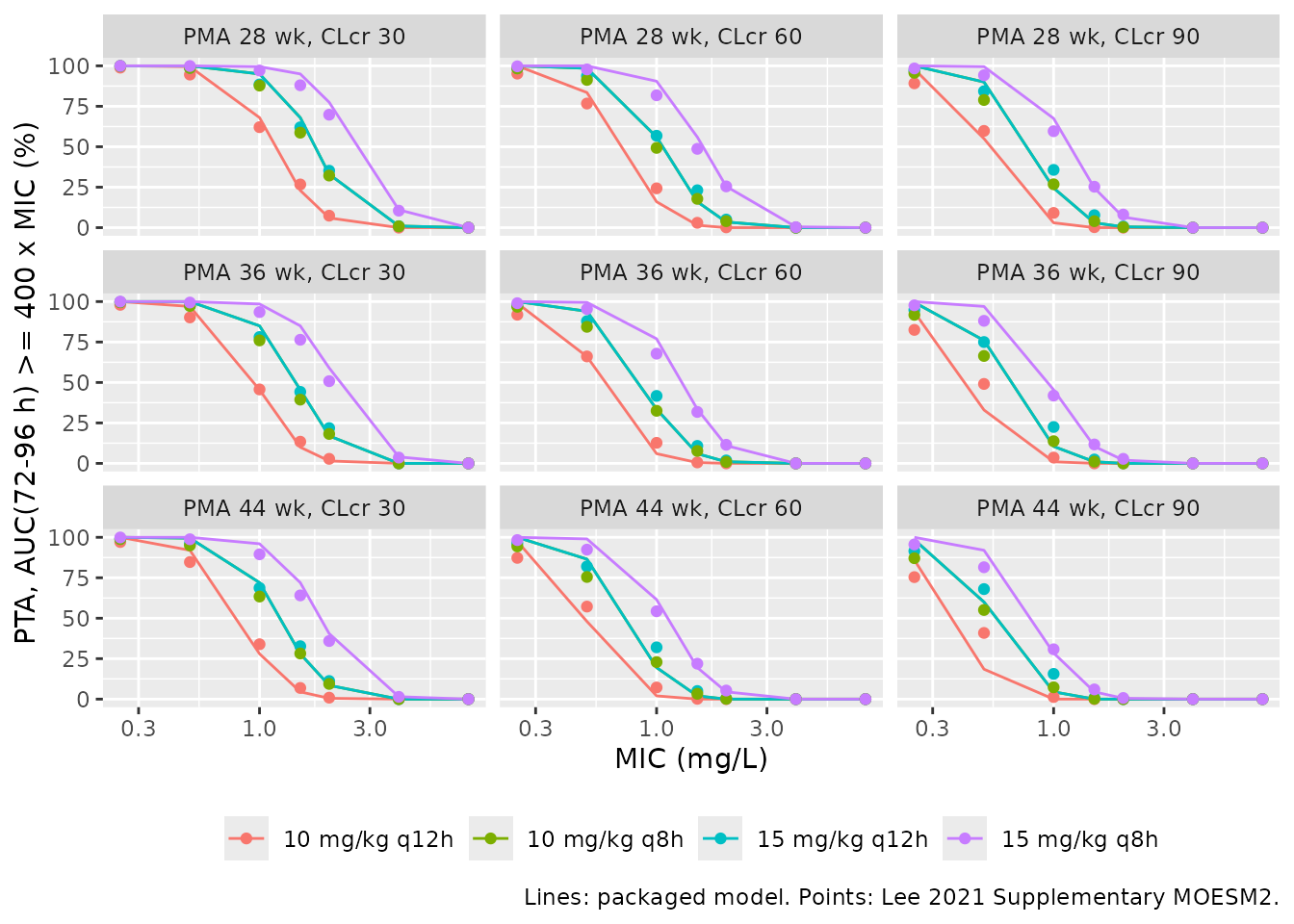
The comparison is made only where the published PTA is between 5% and 95%; outside that range every reading of the model gives 0% or 100%, so those cells test nothing.
inform <- pta_cmp |> dplyr::filter(pta_ge400 > 5, pta_ge400 < 95)
d_ge400 <- inform$sim_ge400 - inform$pta_ge400
c(n_cells = nrow(inform), median_diff = median(d_ge400),
  median_abs_diff = median(abs(d_ge400)), p90_abs_diff = unname(quantile(abs(d_ge400), 0.9)))
#>         n_cells     median_diff median_abs_diff    p90_abs_diff
#>          106.00            2.50            5.95           10.55

inform2 <- pta_cmp |> dplyr::filter(pta_400_600 > 5)
d_400_600 <- inform2$sim_400_600 - inform2$pta_400_600
c(n_cells = nrow(inform2), median_diff = median(d_400_600),
  median_abs_diff = median(abs(d_400_600)))
#>         n_cells     median_diff median_abs_diff
#>             117              -1               4

stopifnot(
  nrow(inform) >= 20,
  # Structural: a mis-transcribed clearance, exponent, reference value or
  # unit moves the whole AUC distribution and shifts every cell together.
  abs(median(d_ge400)) < 5,
  median(abs(d_ge400)) < 10,
  quantile(abs(d_ge400), 0.9) < 20
)
The packaged model reproduces the centre of the published PTA tables. Where the published PTA is between 30% and 70%, the simulated value is within a couple of percentage points of it. The published tables are slightly wider in the tails, though. Where MOESM2 reports 70-95% the model gives a few points more (median about +7), and where it reports 5-30% the model gives a few points less (median about -2). A slightly wider AUC distribution than a clearance variance of 0.123 implies would do this, as if the published simulation carried extra variability. The supplement does not describe its simulation settings, so the source cannot be identified. The model is not tuned to it. The difference is far smaller than the standard-deviation reading of the omegas would produce, and the median AUC, which is set by the structural model and covariates, is reproduced.
Steady-state profiles and PKNCA
Typical-value steady-state profiles are simulated for three neonates
spanning the cohort, all on 10 mg/kg as a 1 h infusion every 12 h (the
most common regimen in the study). NCA is run with PKNCA over the tenth
dosing interval. For a linear one-compartment model at steady state,
AUCtau x CL = dose holds exactly, and that identity is
asserted.
ss_cov <- tibble::tibble(
  treatment = c("Preterm: 1.0 kg, PMA 28 wk, CLcr 25",
                "Median: 1.8 kg, PMA 35.6 wk, CLcr 50.3",
                "Term: 3.5 kg, PMA 42 wk, CLcr 90"),
  WT = c(1.0, 1.8, 3.5), PAGE = c(28, 35.6, 42), CRCL = c(25, 50.3, 90)
) |>
  dplyr::mutate(id = dplyr::row_number())

tau_ss <- 12
n_dose <- 10
obs_grid <- sort(unique(c(seq(0, n_dose * tau_ss, by = 0.25))))

ss_events <- dplyr::bind_rows(
  ss_cov |>
    dplyr::cross_join(tibble::tibble(time = seq(0, (n_dose - 1) * tau_ss, by = tau_ss))) |>
    dplyr::mutate(evid = 1L, amt = 10 * WT, dur = 1, cmt = "central"),
  ss_cov |>
    dplyr::cross_join(tibble::tibble(time = obs_grid)) |>
    dplyr::mutate(evid = 0L, amt = 0, dur = NA_real_, cmt = "central")
) |>
  dplyr::arrange(id, time, dplyr::desc(evid))

ss_sim <- as.data.frame(rxode2::rxSolve(mod_typ, ss_events, returnType = "data.frame",
                                        keep = c("treatment", "WT")))
#> ℹ omega/sigma items treated as zero: 'etalcl', 'etalvc'
#> Warning: multi-subject simulation without without 'omega'

ggplot(ss_sim, aes(time, Cc, colour = treatment)) +
  geom_line() +
  geom_hline(yintercept = c(5, 15), linetype = "dashed", colour = "grey50") +
  labs(x = "Time (h)", y = "Vancomycin (mg/L)", colour = NULL,
       caption = "Typical-value profiles; dashed lines: trough range 5-15 mg/L suggested by Lee 2021.") +
  theme(legend.position = "bottom", legend.direction = "vertical")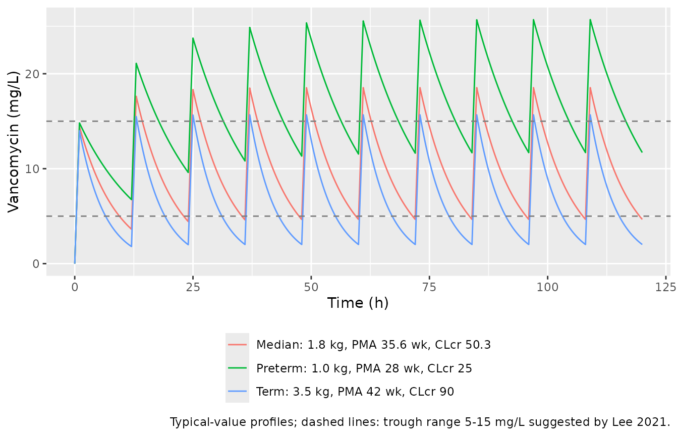
t_start <- (n_dose - 1) * tau_ss
t_end <- n_dose * tau_ss

sim_nca <- ss_sim |>
  dplyr::filter(!is.na(Cc)) |>
  dplyr::select(id, time, Cc, treatment)
sim_nca <- dplyr::bind_rows(
  sim_nca,
  sim_nca |> dplyr::distinct(id, treatment) |> dplyr::mutate(time = 0, Cc = 0)
) |>
  dplyr::distinct(id, treatment, time, .keep_all = TRUE) |>
  dplyr::arrange(id, treatment, time)

dose_df <- ss_events |>
  dplyr::filter(evid == 1L) |>
  dplyr::select(id, time, amt, treatment)

conc_obj <- PKNCA::PKNCAconc(sim_nca, Cc ~ time | treatment + id)
dose_obj <- PKNCA::PKNCAdose(dose_df, amt ~ time | treatment + id)
intervals <- data.frame(start = t_start, end = t_end,
                        cmax = TRUE, tmax = TRUE, cmin = TRUE, auclast = TRUE)
nca_res <- PKNCA::pk.nca(PKNCA::PKNCAdata(conc_obj, dose_obj, intervals = intervals))

nca_wide <- as.data.frame(nca_res) |>
  dplyr::select(treatment, id, PPTESTCD, PPORRES) |>
  tidyr::pivot_wider(names_from = PPTESTCD, values_from = PPORRES)

nca_wide |>
  dplyr::select(treatment, cmax, tmax, cmin, auclast) |>
  dplyr::rename("Neonate" = treatment, "Cmax (mg/L)" = cmax, "Tmax (h)" = tmax,
                "Cmin (mg/L)" = cmin, "AUCtau (mg*h/L)" = auclast) |>
knitr::kable(digits = 2)| Neonate | Cmax (mg/L) | Tmax (h) | Cmin (mg/L) | AUCtau (mg*h/L) |
|---|---|---|---|---|
| Median: 1.8 kg, PMA 35.6 wk, CLcr 50.3 | 18.54 | 1 | 4.66 | 122.29 |
| Preterm: 1.0 kg, PMA 28 wk, CLcr 25 | 25.70 | 1 | 11.70 | 214.50 |
| Term: 3.5 kg, PMA 42 wk, CLcr 90 | 15.67 | 1 | 2.01 | 82.27 |
ss_par <- ss_sim |>
  dplyr::group_by(id) |>
  dplyr::summarise(cl = dplyr::first(cl), vc = dplyr::first(vc),
                   WT = dplyr::first(WT), .groups = "drop") |>
  dplyr::mutate(kel = cl / vc)

# Accumulation after 9 doses relative to true steady state, analytically.
ss_par <- ss_par |>
  dplyr::mutate(frac_ss = 1 - exp(-kel * (n_dose - 1) * tau_ss))

id_chk <- nca_wide |>
  dplyr::inner_join(ss_par, by = "id") |>
  dplyr::mutate(ratio = auclast * cl / (10 * WT))
knitr::kable(dplyr::select(id_chk, treatment, frac_ss, ratio), digits = 4)| treatment | frac_ss | ratio |
|---|---|---|
| Median: 1.8 kg, PMA 35.6 wk, CLcr 50.3 | 1.0000 | 0.9999 |
| Preterm: 1.0 kg, PMA 28 wk, CLcr 25 | 0.9996 | 0.9998 |
| Term: 3.5 kg, PMA 42 wk, CLcr 90 | 1.0000 | 0.9998 |
Assumptions and deviations
-
Omega scale. Table 2 does not say whether its
omegas are variances or standard deviations. The variance reading is
taken because it reproduces the supplementary PTA tables and the
standard-deviation reading does not (see above). NONMEM also reports
$OMEGAelements as variances. -
CL-V covariance. The final model estimates a CL-V
covariance (Results; MOESM3
$OMEGA BLOCK(2)), but the paper does not print it. It is the one value in the packaged model that does not come from Table 2. The correlation (0.48) was profiled on the deposited dataset with every Table 2 value held fixed, and applied to the Table 2 variances. A free re-estimation gives 0.51. - Residual error kept as printed despite the data. The deposited dataset supports a proportional residual SD of about 0.39 rather than the printed 0.583 (111 objective-function points, see above). The printed value is kept because it is the published estimate and the reason for the difference is unknown. Users simulating observed concentrations may prefer the re-estimated pair (additive 2.92 mg/L, proportional 0.386).
- Covariate reference values. The PMA reference of 31.7 weeks is not the per-subject Table 1 median of 35.6 weeks. It equals the median PMA over the records of the deposited dataset (31.69), and 50.3 mL/min/1.73 m^2 is likewise both the Table 1 and the record median of CLcr. Both are kept as printed in Equation (1).
-
PMA units. The paper, and this model’s
PAGEcolumn, use weeks, not the register’s default of months. -
Weight exponents. Both are fixed, not estimated
(Abstract; MOESM3 hard-codes 0.75 and 1), and are wrapped in
fixed(). -
Residual error form. MOESM3 writes the combined
error with the additive and proportional SDs as thetas adding in
variance (
SIGMA 1 FIX). That is nlmixr2’s default combination forprop() + add(). - Below-quantification values. The paper kept them as observed values (Methods). This does not affect simulation.
- PTA simulation settings. MOESM1 and MOESM2 do not state the virtual cohort size or whether residual error or the CL-V correlation were used. Neither of the last two changes the AUC distribution materially, because AUC over a steady-state window depends on clearance alone. The residual agreement is described in the PTA section.
- Errata. No erratum or correction was found on the publisher’s page or in PubMed (checked 2026-09-28).