Lamotrigine (Hussein 1997)
Source:vignettes/articles/Hussein_1997_lamotrigine.Rmd
Hussein_1997_lamotrigine.RmdModel and source
- Citation: Hussein Z, Posner J. Population pharmacokinetics of lamotrigine monotherapy in patients with epilepsy: retrospective analysis of routine monitoring data. Br J Clin Pharmacol. 1997;43(5):457-465.
- Article: https://doi.org/10.1046/j.1365-2125.1997.00594.x
- Population PK developed by retrospective analysis of plasma lamotrigine drug-monitoring concentrations collected in three multicentre Phase II/III trials of lamotrigine monotherapy in patients with newly diagnosed epilepsy.
- Source files on disk:
from_people/literature_2018_search/Hussein_1997_Population_pharmacokinetics_of_lamotrigi_7c3595.pdf.
The packaged model Hussein_1997_lamotrigine is a
one-compartment open model with first-order absorption, a first-order
auto-induction term on apparent oral clearance, and a multiplicative
race effect on CL_o for Asian vs Caucasian patients. Apparent volume of
distribution and absorption rate constant are time-invariant and carry
no covariate effects in the final model.
Population
The published model was fit to 163 patients (158 Caucasians + 5 Asians; 81 males + 82 females; ages 14-76 years; weight 40.5-106.5 kg; mean weight roughly 68 kg) drawn from three GlaxoWellcome Phase II/III monotherapy trials. Twenty Caucasian females received concomitant oral contraceptives. Inclusion required newly diagnosed partial or generalised tonic-clonic epilepsy, no prior antiepileptic-drug exposure, and normal hepatic and renal function. Plasma samples were collected as routine drug-monitoring concentrations at the end of treatment weeks 1, 2, 4, 6, 8, 12, 18, 24, and 48 (Hussein 1997 Methods, p. 458; demographic distributions in Figure 1, p. 459).
The structured demographics are also embedded in the model file as a
population list
(inst/modeldb/specificDrugs/Hussein_1997_lamotrigine.R)
alongside the per-covariate covariateData block and the
covariatesDataExcluded register of
screened-but-not-retained covariates.
Source trace
The per-parameter origin is recorded as an in-file comment next to
each ini() entry in
inst/modeldb/specificDrugs/Hussein_1997_lamotrigine.R. The
table below collects them in one place for review.
| Equation / parameter | Value | Source location |
|---|---|---|
| Structural form: one-compartment with first-order absorption and elimination | n/a | Hussein 1997 Methods ‘Pharmacokinetic analyses’, p. 458 |
| Auto-induction equation TVCL = theta_CL - theta_CL^TIME1 * exp(-theta_CL^TIME2 * TIME) | n/a | Hussein 1997 Results ‘Population pharmacokinetics’, equation listed on p. 459 |
Final CL_o equation TVCL = theta_CL * (1 + RACE * theta_ASIANS_CL) *
(1 - (theta_CL^TIME1/theta_CL) * exp(-theta_CL^TIME2 * TIME)) factored
equivalently as
(cl_ss - cl_time * exp(-kdes * time_wk)) * (1 + e_race_asian_cl * RACE_ASIAN)
|
n/a | Hussein 1997 Table 4 ‘Structural models’ block, p. 464 |
lcl_ss -> exp = 2.28 L/h |
2.28 | Table 4 row ‘Oral clearance (CL_o)’ theta_CL, p. 464 |
lcl_time -> exp = 0.338 L/h |
0.338 | Table 4 row ‘Effect of duration of therapy on CL_o’ theta_CL^TIME1, p. 464 |
lkdes -> exp = 0.119 /week |
0.119 | Table 4 row ‘Effect of duration of therapy on CL_o’ theta_CL^TIME2, p. 464 |
lvc -> exp = 77.4 L |
77.4 | Table 4 row ‘Apparent volume of distribution (V/F)’ theta_V, p. 464 |
lka -> exp = 3.18 /h |
3.18 | Table 4 row ‘First-order absorption rate constant (K_a)’ theta_Ka, p. 464 |
e_race_asian_cl (Asian effect on CL_o) |
-0.287 | Table 4 row ‘Effect of Asians on CL_o’ theta_CL^ASIANS, p. 464 |
etalcl IIV (CV 32.1%; omega^2 = log(1+0.321^2) =
0.0981) |
0.0981 | Table 4 row ‘CV for interpatient variability in CL_o’, p. 464 |
etalvc IIV (CV 33.6%; omega^2 = log(1+0.336^2) =
0.1070) |
0.1070 | Table 4 row ‘CV for interpatient variability in V/F’, p. 464 |
propSd (CV 20.8%) |
0.208 | Table 4 row ‘CV for residual variability’ sigma^2, p. 464 |
| Random-effects form CL_o = TVCL * (1 + eta_CL), V/F = TVV * (1 + eta_V) | translated to log-normal | Table 4 ‘random effects models’ block, p. 464; see Assumptions and deviations below |
| Residual form Cobs = Cpred * (1 + epsilon) | proportional | Table 4 ‘random effects models’ block, p. 464 |
Virtual cohort
Original observed concentrations are not publicly available. The figures below use virtual populations whose covariate distributions approximate the published trial demographics (Hussein 1997 Results ‘Demographic characteristics’, p. 459):
- 97% Caucasian, 3% Asian (RACE_ASIAN as 0/1 indicator).
- Body weight is not used in the final model; it is retained on the event table for documentation only.
set.seed(773L)

n_per_arm <- 100L

subjects <- bind_rows(
  tibble::tibble(id = seq_len(n_per_arm),                RACE_ASIAN = 0L, cohort = "Caucasian"),
  tibble::tibble(id = n_per_arm + seq_len(n_per_arm),    RACE_ASIAN = 1L, cohort = "Asian")
)

# Daily 200-mg doses for 48 weeks.
dose_times <- seq(0, 48 * 7 * 24 - 24, by = 24)
# Sampling: weekly trough snapshot to visualise the auto-induction trajectory,
# plus a dense final-week PK profile for the steady-state NCA.
obs_times <- sort(unique(c(
  seq(0.5, 48 * 7 * 24, by = 24 * 7),                   # weekly snapshots
  48 * 7 * 24 - 24 + c(0.5, 1, 2, 4, 6, 12, 24)         # rich last-interval profile
)))

doses_df <- tidyr::crossing(subjects, time = dose_times) |>
  mutate(amt = 200, cmt = "depot", evid = 1L)

obs_df <- tidyr::crossing(subjects, time = obs_times) |>
  mutate(amt = 0, cmt = NA_character_, evid = 0L)

events <- bind_rows(doses_df, obs_df) |>
  arrange(id, time, desc(evid))

stopifnot(!anyDuplicated(unique(events[, c("id", "time", "evid")])))
Simulation
mod <- readModelDb("Hussein_1997_lamotrigine")

# Stochastic VPC simulation including between-subject variability. rxSolve
# returns observation rows only (dose rows are dropped); the `keep =` block
# carries the cohort label through onto every observation row.
sim <- rxode2::rxSolve(
  mod,
  events = events,
  keep   = c("cohort"),
  returnType = "data.frame"
)
#> ℹ parameter labels from comments will be replaced by 'label()'
sim$cohort <- factor(sim$cohort, levels = c("Caucasian", "Asian"))
sim$time_wk <- sim$time / 168
# Deterministic typical-value trajectory for the auto-induction line in
# Figure 5 -- zero out the random effects so we get the population TVCL(t).
mod_typical <- rxode2::zeroRe(mod)
#> ℹ parameter labels from comments will be replaced by 'label()'
sim_typ <- rxode2::rxSolve(
  mod_typical,
  events = events,
  keep   = c("cohort"),
  returnType = "data.frame"
)
#> ℹ omega/sigma items treated as zero: 'etalcl', 'etalvc'
#> Warning: multi-subject simulation without without 'omega'
sim_typ$cohort <- factor(sim_typ$cohort, levels = c("Caucasian", "Asian"))
sim_typ$time_wk <- sim_typ$time / 168
Replicate published figures
Figure 5 – CL_o vs duration of therapy
Hussein 1997 Figure 5 (p. 464) plots NONMEM empirical Bayes estimates of individual oral clearance against duration of therapy in weeks, overlaid with the typical-value population curve from the final model. The Caucasian typical-value line rises from 1.94 L/h at week 0 to 2.28 L/h by week 48 (a 17.5% increase); the Asian typical-value line tracks 28.7% lower at every time point.
typ_cl <- sim_typ |>
  group_by(cohort, time_wk) |>
  summarise(cl_typical = mean(cl), .groups = "drop")

ind_cl <- sim |>
  group_by(cohort, time_wk) |>
  summarise(
    Q05 = quantile(cl, 0.05, na.rm = TRUE),
    Q50 = quantile(cl, 0.50, na.rm = TRUE),
    Q95 = quantile(cl, 0.95, na.rm = TRUE),
    .groups = "drop"
  )

ggplot(ind_cl, aes(time_wk, Q50, colour = cohort, fill = cohort)) +
  geom_ribbon(aes(ymin = Q05, ymax = Q95), alpha = 0.15, colour = NA) +
  geom_line(data = typ_cl, aes(time_wk, cl_typical, colour = cohort),
            linewidth = 1.0) +
  geom_hline(yintercept = c(1.94, 2.28), linetype = "dashed",
             colour = "grey60", linewidth = 0.4) +
  annotate("text", x = 5, y = 1.94, label = "1.94 L/h (Caucasian wk 0)",
           vjust = -0.6, hjust = 0, colour = "grey40", size = 3) +
  annotate("text", x = 30, y = 2.28, label = "2.28 L/h (Caucasian wk 48)",
           vjust = 1.4, hjust = 0, colour = "grey40", size = 3) +
  scale_x_continuous(breaks = seq(0, 48, by = 8)) +
  labs(
    x = "Time since start of therapy (weeks)",
    y = expression(paste("Oral clearance ", CL[o], " (L/h)")),
    colour = "Cohort", fill = "Cohort",
    title = "Figure 5 -- Auto-induction of apparent oral clearance",
    caption = "Replicates Figure 5 of Hussein 1997 (typical-value population line) plus a stochastic 5-95% interval."
  ) +
  theme_minimal()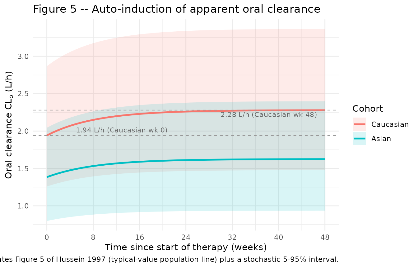
The typical-value lines reproduce the published numbers exactly:
typ_cl |>
  mutate(time_wk_grouping = case_when(
    time_wk < 0.05                       ~ "week 0",
    abs(time_wk - 48)  < 0.05             ~ "week 48",
    TRUE                                  ~ NA_character_
  )) |>
  filter(!is.na(time_wk_grouping)) |>
  arrange(cohort, time_wk_grouping) |>
  select(cohort, time_wk_grouping, cl_typical) |>
  knitr::kable(
    digits = 3,
    caption = "Typical-value CL_o at start of therapy and at 48 weeks (compare to Hussein 1997 Table 4 + Discussion: Caucasian 1.94 -> 2.28 L/h; Asian 1.39 -> 1.63 L/h)."
)| cohort | time_wk_grouping | cl_typical |
|---|---|---|
| Caucasian | week 0 | 1.942 |
| Caucasian | week 48 | 2.279 |
| Asian | week 0 | 1.385 |
| Asian | week 48 | 1.625 |
Population elimination half-life
Hussein 1997 Discussion (p. 464) reports the typical-value elimination half-life from t_{1/2} = ln(2) * V/F / CL_o: 27.6 h in Caucasians at week 0 declining to 23.5 h by week 48 (14.8% reduction), and 38.7 h in Asians at week 0 declining to 33.0 h by week 48 (same fractional reduction). Our typical-value trajectory reproduces these numbers:
typ_cl |>
  mutate(time_wk_grouping = case_when(
    time_wk < 0.05                       ~ "week 0",
    abs(time_wk - 48)  < 0.05             ~ "week 48",
    TRUE                                  ~ NA_character_
  )) |>
  filter(!is.na(time_wk_grouping)) |>
  mutate(
    t_half_h = log(2) * 77.4 / cl_typical
  ) |>
  arrange(cohort, time_wk_grouping) |>
  select(cohort, time_wk_grouping, cl_typical, t_half_h) |>
  knitr::kable(
    digits = 2,
    caption = "Typical-value elimination half-life (compare to Hussein 1997 Discussion: Caucasian 27.6 -> 23.5 h; Asian 38.7 -> 33.0 h)."
)| cohort | time_wk_grouping | cl_typical | t_half_h |
|---|---|---|---|
| Caucasian | week 0 | 1.94 | 27.62 |
| Caucasian | week 48 | 2.28 | 23.54 |
| Asian | week 0 | 1.38 | 38.74 |
| Asian | week 48 | 1.62 | 33.02 |
PKNCA validation
The Hussein 1997 paper does not tabulate NCA parameters directly; instead it reports the underlying population PK parameters (CL_o, V/F, K_a) and the implied elimination half-life. We use PKNCA to compute steady-state NCA parameters from a multidose simulation over the final week of therapy (week 48), when the auto-induction is essentially complete, and compare them back to the published structural values via the closed-form relationships AUC_ss = Dose / CL_o (per dosing interval), C_avg = AUC_ss / tau, and t_{1/2} = ln(2) * V/F / CL_o.
sim_ss <- sim |>
  filter(time >= (47 * 7 * 24), time <= (48 * 7 * 24))

conc_obj <- PKNCA::PKNCAconc(
  sim_ss |> select(id, time, Cc, cohort),
  Cc ~ time | cohort + id,
  concu = "mg/L", timeu = "h"
)

dose_df <- events |>
  filter(evid == 1) |>
  group_by(id) |>
  filter(time == max(time)) |>   # final dose, used as the SS dose anchor
  ungroup() |>
  select(id, time, amt, cohort)

dose_obj <- PKNCA::PKNCAdose(
  dose_df, amt ~ time | cohort + id,
  doseu = "mg"
)

tau <- 24
start_ss <- min(dose_df$time)
end_ss   <- start_ss + tau

intervals <- data.frame(
  start    = start_ss,
  end      = end_ss,
  cmax     = TRUE,
  cmin     = TRUE,
  cav      = TRUE,
  tmax     = TRUE,
  auclast  = TRUE,
  half.life = TRUE
)

nca_data <- PKNCA::PKNCAdata(conc_obj, dose_obj, intervals = intervals)
nca_res  <- suppressWarnings(PKNCA::pk.nca(nca_data))

nca_summary <- summary(nca_res)
knitr::kable(
  nca_summary,
  caption = "Simulated steady-state NCA parameters (last dosing interval, 200 mg QD)."
)| Interval Start | Interval End | cohort | N | AUClast (h*mg/L) | Cmax (mg/L) | Cmin (mg/L) | Tmax (h) | Cav (mg/L) | Half-life (h) |
|---|---|---|---|---|---|---|---|---|---|
| 8040 | 8064 | Asian | 100 | NC | 6.58 [27.3] | 3.99 [42.1] | 1.00 [1.00, 1.00] | NC | 36.9 [17.3] |
| 8040 | 8064 | Caucasian | 100 | NC | 5.10 [22.0] | 2.65 [39.4] | 1.00 [1.00, 1.00] | NC | 27.8 [11.6] |
Comparison against structural relationships
Closed-form expectations from the typical-value population model at the end of therapy (week 48):
- Caucasian CL_o,ss = 2.28 L/h, V/F = 77.4 L
- C_avg,ss = 200 mg / (2.28 L/h * 24 h) = 3.655 mg/L
- t_{1/2} = ln(2) * 77.4 / 2.28 = 23.5 h
- Asian CL_o,ss = 2.28 * (1 - 0.287) = 1.626 L/h, V/F = 77.4 L
- C_avg,ss = 200 / (1.626 * 24) = 5.125 mg/L
- t_{1/2} = ln(2) * 77.4 / 1.626 = 33 h
The PKNCA cav and half.life columns in the
table above should fall within a few percent of these closed-form
values; the small residual gap reflects incomplete steady state (week 48
reaches ~94% of asymptotic CL after auto- induction) and the C_avg
averaging interval.
Assumptions and deviations
-
IIV reparameterisation (additive-on-fraction ->
log-normal). Hussein 1997 encodes between-subject variability
as
CL_oj = TVCL * (1 + eta_CLj)with eta_CL ~ N(0, omega^2) (Table 4 ‘random effects models’ block, p. 464). The canonical nlmixr2lib form is log-normalCL_oj = TVCL * exp(eta_CLj). The two parameterisations are within ~5% of each other for the published magnitudes (CV 32% on CL, 34% on V/F); the log-normal omega^2 values used inini()arelog(1 + CV^2)(= 0.0981 for CL and 0.1070 for V/F). Seeparameter-names.md-> “Inter-individual variability”. -
Single composite eta on CL. The paper reports one
eta on the composite CL_o that scales the entire TVCL(t) trajectory in
lockstep (i.e., the same random effect multiplies both the asymptotic
and the time-decaying arms). We encode this with a single
etalcldeclared viapaper_specific_etasand applied identically to bothlcl_ssandlcl_timeinsidemodel(). -
TIME interpretation. TIME in the auto-induction
term is duration of therapy in weeks since the first dose. In the model
file we use the rxode2 simulation time
time(in hours) and convert viatime_wk <- time / 168. The auto-induction term therefore depends only on time since the simulation start; if a real dataset has a baseline time offset (i.e., time 0 is not the first dose), the user must subtract that offset before passing torxSolve. - No absorption IIV. Hussein 1997 Discussion (p. 462) notes that the magnitude of variability in K_a was “inestimable since few plasma concentrations were collected during the absorption phase”. We follow the paper and do not estimate IIV on K_a.
- Dosing intervals assumed. The paper records exact times only for the last dose prior to each clinic visit; dosing intervals of 24, 12, and 8 h were assumed for once/twice/thrice daily regimens (Methods ‘Database construction’, p. 458). This is an assumption of the published fit, not an additional simplification introduced in nlmixr2lib.
-
Covariates screened but not retained. Body weight,
age, female sex, oral contraceptive use, and total daily dose were each
tested in univariate and multivariate analyses (Tables 1-3) and dropped
from the final model. The packaged model records these in
covariatesDataExcludedfor provenance; the final model uses only TIME (auto-induction) and RACE_ASIAN. - Small Asian-cohort caution. Only 5 of 163 patients were Asian. Hussein 1997 Discussion (p. 464) cautions that the 28.7% lower CL_o in Asians should be interpreted carefully given the small N; we carry the published point estimate without alteration but note that downstream simulations with the Asian covariate may carry meaningful uncertainty beyond what the 95% CI alone conveys.