Model and source
- Citation: Kim JH, Han N, Kim MG, Yun H-Y, Lee S, Bae E, Kim YS, Kim I-W, Oh JM. Increased Exposure of Tacrolimus by Co-administered Mycophenolate Mofetil: Population Pharmacokinetic Analysis in Healthy Volunteers. Sci Rep. 2018;8:1687. doi:10.1038/s41598-018-20071-3.
- Description: Integrated population PK model of the tacrolimus (TAC) - mycophenolate mofetil (MMF) drug-drug interaction in healthy Korean male volunteers (Kim 2018, final integrated model). TAC follows a two-compartment model with first-order absorption and a lag time; apparent oral clearance (CL/F) is increased 1.48-fold in CYP3A5 expressers and is suppressed by co-administered mycophenolic acid (MPA) through an inverse-exponential interaction (CL/F = 13.8 / exp(0.0294Cmpa) 1.48^CYP3A5). MPA (the active moiety of MMF) follows a two-compartment model with first-order absorption; MPA is metabolised to MPAG (7-O-glucuronide; 85% of metabolism) and AcMPAG (acyl glucuronide; 15%). MPAG undergoes enterohepatic recirculation via a gallbladder compartment that empties into the MPA absorption compartment during a meal-triggered window. Tacrolimus concentrations are in ng/mL; MPA, MPAG and AcMPAG are in ug/mL.
- Article: https://doi.org/10.1038/s41598-018-20071-3
This is the final integrated model of Kim et al. (2018), which jointly describes tacrolimus (TAC) and the mycophenolate mofetil (MMF) metabolite cascade – mycophenolic acid (MPA), MPA 7-O-glucuronide (MPAG), and MPA acyl glucuronide (AcMPAG) – and quantifies the TAC-MMF drug-drug interaction. The independent (TAC-alone / MMF-alone) models in Table 3 are intermediate development steps and are not packaged separately.
Population
The model was developed from a three-period, fixed-sequence, open-label, single-dose drug-drug-interaction study in 17 healthy Korean male volunteers (NCT02743247; conducted 2015-2016). Subjects received 1,000 mg MMF alone, then 5 mg TAC alone, then the 1,000 mg MMF + 5 mg TAC combination, with one-week washout periods. Median age was 25 years (range 20-42), median weight 69.7 kg (57.4-88.3 kg), and all subjects were of Korean ethnicity with normal renal and hepatic function (Table 1). Four of 17 subjects (23.5%) were CYP3A5 expressers (CYP3A51/1 or CYP3A51/3). Because baseline demographic variation was small, the CYP3A5 genotype was the only covariate retained in the final model.
The same information is available programmatically via
readModelDb("Kim_2018_tacrolimus")$population.
Source trace
Per-parameter origin is recorded as an in-file comment next to each
ini() entry in
inst/modeldb/specificDrugs/Kim_2018_tacrolimus.R. All
structural estimates are the Integrated model column of
Kim 2018 Table 3.
| Equation / parameter | Value | Source location |
|---|---|---|
lka (Ka TAC) |
1.78 1/h | Table 3, Ka TAC (integrated) |
lcl (CL/F TAC, typical) |
13.8 L/h | Table 3, CL/F TAC (integrated) |
lvc (V2/F TAC) |
93 L | Table 3, V2/F (integrated) |
lk23, lk32 (TAC distribution) |
0.313, 0.0719 1/h | Table 3, k23 / k32 (integrated) |
ltlag (TAC lag time) |
0.59 h | Table 3, Lag time (integrated) |
e_cyp3a5_cl (CYP3A5 on CL/F) |
1.48 | Table 3 + equation (2) |
e_cmpa_cl (MPA-TAC interaction slope) |
0.0294 mL/ug | Table 3, Interaction + equation (2) |
lka_mpa (Ka MPA) |
2.29 1/h | Table 3, Ka MPA (integrated) |
lcl_mpa (CL/F MPA) |
16.3 L/h | Table 3, CL/F MPA (integrated) |
lvc_mpa (V5/F MPA) |
19.7 L | Table 3, V5/F (integrated) |
lk56, lk65 (MPA distribution) |
1.12, 0.131 1/h | Table 3, k56 / k65 (integrated) |
f_mpag (fraction MPA -> MPAG, fixed) |
0.85 | Table 3, fMPA (fixed) |
lvc_mpag (V7/F MPAG) |
5.83 L | Table 3, V7/F (integrated) |
lk70 (MPAG elimination) |
0.251 1/h | Table 3, k70 (integrated) |
lehc (fraction MPAG EHC) |
0.367 | Table 3, EHC + equation (1) |
lk84 (gallbladder emptying) |
18.4 1/h | Table 3, k84 (integrated) |
lmtime1 (meal time) |
7.96 h | Table 3, MTIME1 (integrated) |
lmtime2 (emptying duration, fixed) |
1.0 h | Table 3, MTIME2 (fixed) |
lvc_acmpag (V9/F AcMPAG, fixed) |
23 L | Table 3, V9/F (fixed) |
lk90 (AcMPAG elimination, fixed) |
2.15 1/h | Table 3, k90 (fixed) |
| Residual error (TAC / MPA / MPAG / AcMPAG) | see ini()
|
Table 3, sigma rows (integrated) |
| IIV (Ka/CL/V TAC; Ka/CL/V MPA; EHC) | see ini()
|
Table 3, IIV CV% (integrated) |
d/dt(...) 9-compartment structure |
n/a | Figure 1 (model schematic) |
k57 = fMPA*CL_MPA/V5;
k59 = (1-fMPA)*CL_MPA/V5
|
derived | Figure 1 (MPA exits only via k57/k59) |
k78 = EHC*k70/(1-EHC) |
derived | equation (1) |
The metabolite-formation rate constants k57 (MPA ->
MPAG) and k59 (MPA -> AcMPAG) and the biliary-transfer
constant k78 (MPAG -> gallbladder) are not tabulated in
Table 3. They are recovered algebraically from the Figure 1 structure:
MPA central is eliminated solely through metabolism, so
k57 + k59 = CL/F_MPA / V5/F, split by the fixed fraction
fMPA = 0.85; and equation (1),
EHC = k78 / (k70 + k78), inverts to
k78 = EHC*k70/(1-EHC).
Virtual cohort
Original observed data are not publicly available. The figures below use a virtual population matching the published CYP3A5 expresser frequency (23.5%); the model carries no continuous demographic covariate, so weight/age are not needed for simulation. Two treatment arms reproduce the study’s interaction contrast: TAC alone (5 mg) and TAC + MMF (5 mg TAC + 1,000 mg MMF).
set.seed(20180120)

n_per_arm <- 250L
obs_times <- sort(unique(c(seq(0, 12, by = 0.25), seq(12, 72, by = 1))))

make_cohort <- function(n, arm, with_mmf, id_offset = 0L) {
  cyp <- stats::rbinom(n, 1L, 4 / 17)   # 23.5% CYP3A5 expressers (Table 1)
  dplyr::bind_rows(lapply(seq_len(n), function(i) {
    ev <- rxode2::et(amt = 5, cmt = "depot", time = 0)
    if (with_mmf) ev <- rxode2::et(ev, amt = 1000, cmt = "depot_mpa", time = 0)
    ev <- rxode2::et(ev, obs_times, cmt = "Cc")
    df <- as.data.frame(ev)
    df$id <- id_offset + i
    df$arm <- arm
    df$CYP3A5_EXPR <- cyp[i]
    df
  }))
}

events <- dplyr::bind_rows(
  make_cohort(n_per_arm, "TAC alone",  with_mmf = FALSE, id_offset = 0L),
  make_cohort(n_per_arm, "TAC + MMF",  with_mmf = TRUE,  id_offset = n_per_arm)
)
stopifnot(!anyDuplicated(unique(events[, c("id", "time", "evid")])))
Simulation
mod <- readModelDb("Kim_2018_tacrolimus")

# Stochastic simulation (between-subject variability) for the VPC bands.
sim <- rxode2::rxSolve(mod, events = events,
                       keep = c("arm", "CYP3A5_EXPR"),
                       returnType = "data.frame", addDosing = FALSE,
                       atol = 1e-8, rtol = 1e-6)
#> ℹ parameter labels from comments will be replaced by 'label()'
For the typical-value interaction figure, the random effects are zeroed:
mod_typical <- rxode2::zeroRe(mod)
#> ℹ parameter labels from comments will be replaced by 'label()'

typ_events <- dplyr::bind_rows(
  make_cohort(1L, "TAC alone", with_mmf = FALSE, id_offset = 0L),
  make_cohort(1L, "TAC + MMF", with_mmf = TRUE,  id_offset = 1L)
)
typ_events$CYP3A5_EXPR <- 0   # nonexpresser (majority genotype)

sim_typ <- rxode2::rxSolve(mod_typical, events = typ_events,
                           keep = c("arm"), returnType = "data.frame",
                           addDosing = FALSE)
#> ℹ omega/sigma items treated as zero: 'etalka', 'etalcl', 'etalvc', 'etalka_mpa', 'etalcl_mpa', 'etalvc_mpa', 'etalehc'
#> Warning: multi-subject simulation without without 'omega'
Replicate published figures
Figure 2 – VPC of the four analytes (combination arm)
Kim 2018 Figure 2 shows prediction-corrected VPCs of TAC, MPA, MPAG
and AcMPAG in the combination treatment. Without the observed data we
plot the simulated median and 5th-95th percentile prediction interval
for the TAC + MMF arm.
combo <- dplyr::filter(sim, arm == "TAC + MMF")

vpc_long <- combo |>
  dplyr::select(time, TAC = Cc, MPA = Cc_mpa, MPAG = Cc_mpag, AcMPAG = Cc_acmpag) |>
  tidyr::pivot_longer(-time, names_to = "analyte", values_to = "conc") |>
  dplyr::mutate(analyte = factor(analyte, levels = c("TAC", "MPA", "MPAG", "AcMPAG")))

vpc_bands <- vpc_long |>
  dplyr::group_by(analyte, time) |>
  dplyr::summarise(
    Q05 = quantile(conc, 0.05, na.rm = TRUE),
    Q50 = quantile(conc, 0.50, na.rm = TRUE),
    Q95 = quantile(conc, 0.95, na.rm = TRUE),
    .groups = "drop"
  )

ggplot(vpc_bands, aes(time, Q50)) +
  geom_ribbon(aes(ymin = Q05, ymax = Q95), alpha = 0.25) +
  geom_line() +
  facet_wrap(~analyte, scales = "free_y") +
  labs(x = "Time (h)",
       y = "Concentration (TAC: ng/mL; MPA/MPAG/AcMPAG: ug/mL)",
       title = "Figure 2 -- integrated-model VPC (combination arm)",
       caption = "Replicates Figure 2 of Kim 2018 (predicted median + 5th-95th percentile; observed data not public).") +
  theme_bw()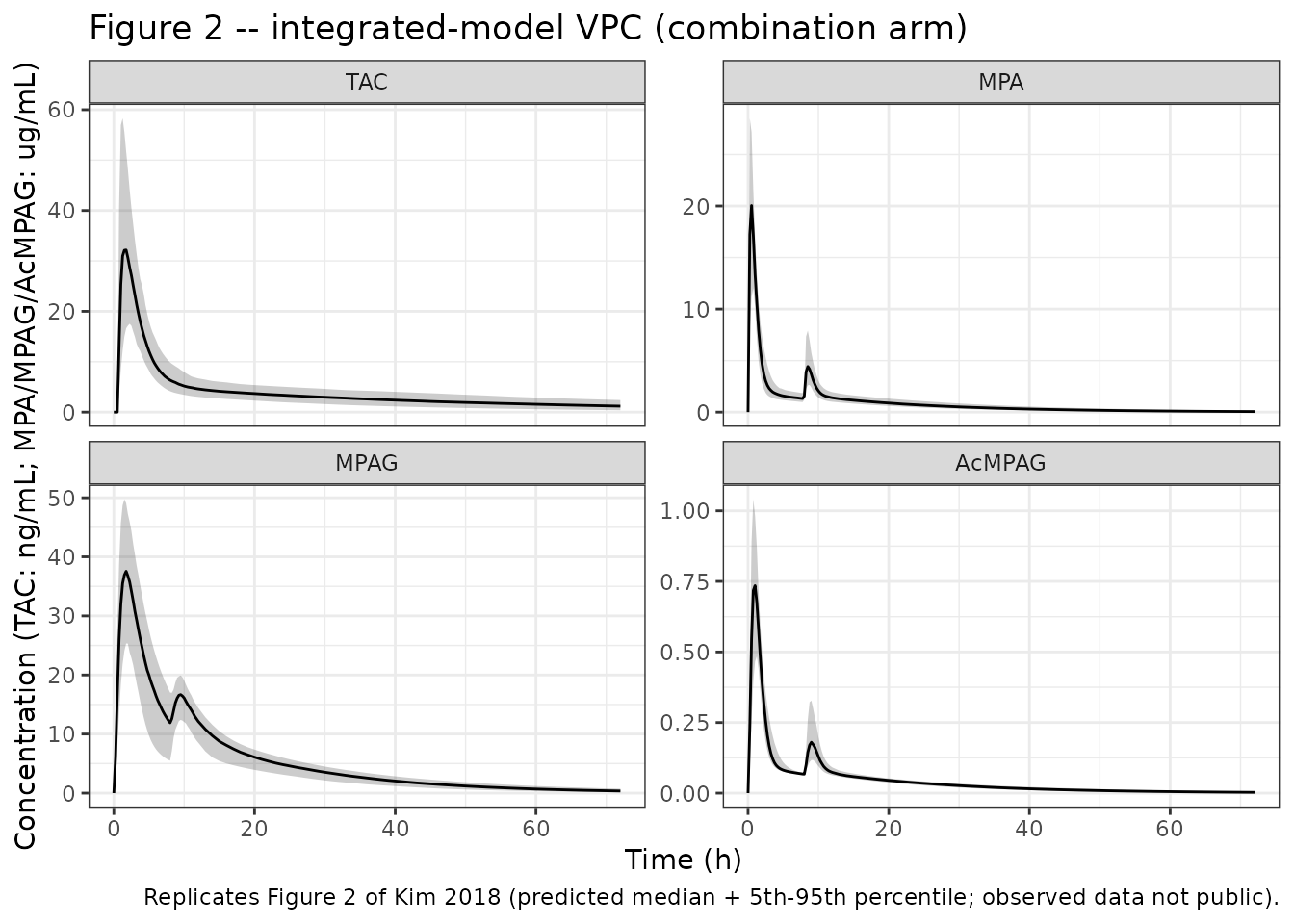
The MPA panel shows the characteristic secondary peak around 8 h driven by the meal-triggered gallbladder emptying (MTIME1 = 7.96 h) that completes the enterohepatic-recirculation loop – matching the “secondary peak at 6-12 h” described in the paper.
Tacrolimus interaction (typical value)
The integrated model encodes the MMF interaction as an inverse-exponential suppression of TAC CL/F by MPA concentration (equation (2)). The typical-value profiles below show the higher TAC exposure when co-administered with MMF.
ggplot(sim_typ, aes(time, Cc, colour = arm)) +
  geom_line(linewidth = 0.9) +
  labs(x = "Time (h)", y = "Tacrolimus (ng/mL)",
       colour = NULL,
       title = "Tacrolimus typical-value profile: alone vs. with MMF",
       caption = "MMF co-administration lowers TAC CL/F (equation (2)), raising exposure.") +
  theme_bw()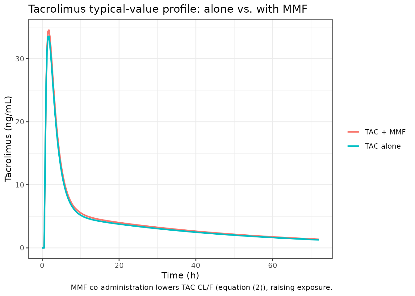
PKNCA validation
NCA parameters for tacrolimus are computed with PKNCA per treatment arm and compared against Kim 2018 Table 2 (TAC alone vs. TAC + MMF).
sim_nca <- sim |>
  dplyr::filter(!is.na(Cc)) |>
  dplyr::select(id, time, Cc, arm)

conc_obj <- PKNCA::PKNCAconc(sim_nca, Cc ~ time | arm + id,
                             concu = "ng/mL", timeu = "hr")

dose_df <- events |>
  dplyr::filter(evid == 1, cmt == "depot") |>   # the tacrolimus dose
  dplyr::select(id, time, amt, arm)

dose_obj <- PKNCA::PKNCAdose(dose_df, amt ~ time | arm + id, doseu = "mg")

intervals <- data.frame(
  start = 0, end = Inf,
  cmax = TRUE, tmax = TRUE, aucinf.obs = TRUE, half.life = TRUE
)

nca_res <- PKNCA::pk.nca(PKNCA::PKNCAdata(conc_obj, dose_obj, intervals = intervals))
knitr::kable(summary(nca_res),
caption = "Simulated tacrolimus NCA by treatment arm.")| Interval Start | Interval End | arm | N | Cmax (ng/mL) | Tmax (hr) | Half-life (hr) | AUCinf,obs (hr*ng/mL) |
|---|---|---|---|---|---|---|---|
| 0 | Inf | TAC + MMF | 250 | 33.7 [37.2] | 1.50 [1.00, 3.50] | 33.4 [12.3] | 354 [30.1] |
| 0 | Inf | TAC alone | 250 | 32.1 [33.6] | 1.50 [0.750, 3.50] | 33.2 [10.6] | 333 [30.9] |
Comparison against published NCA (Table 2)
published <- tibble::tribble(
  ~arm,         ~cmax, ~tmax, ~aucinf.obs,
  "TAC alone",   33.5,   1,    322.4,
  "TAC + MMF",   35.0,   2,    393.6
)

cmp <- nlmixr2lib::ncaComparisonTable(
  simulated     = nca_res,
  reference     = published,
  by            = "arm",
  params        = c("cmax", "tmax", "aucinf.obs"),
  units         = c(cmax = "ng/mL", tmax = "h", aucinf.obs = "ng*h/mL"),
  tolerance_pct = 20
)
knitr::kable(
  cmp,
  caption = paste(
    "Tacrolimus NCA: simulated (median across n =",
    length(unique(sim_nca$id)),
    ") vs. published (Kim 2018 Table 2). * differs from reference by",
    ">20%."
  )
)| NCA parameter | arm | Reference | Simulated | % diff |
|---|---|---|---|---|
| Cmax (ng/mL) | TAC alone | 33.5 | 32.2 | -3.8% |
| Cmax (ng/mL) | TAC + MMF | 35 | 34.3 | -2.0% |
| Tmax (h) | TAC alone | 1 | 1.5 | +50.0%* |
| Tmax (h) | TAC + MMF | 2 | 1.5 | -25.0%* |
| AUC0-∞ (obs) (ng*h/mL) | TAC alone | 322 | 332 | +2.9% |
| AUC0-∞ (obs) (ng*h/mL) | TAC + MMF | 394 | 358 | -9.1% |
The Kim 2018 Table 2 also reports CL/F (TAC alone 20.1 L/h; TAC + MMF 14.2 L/h). The integrated model’s typical CL/F is 13.8 L/h; the TAC + MMF arm matches closely, while the TAC-alone arm runs lower than the independent-model NCA-derived value (see Assumptions and deviations below).
The simulated combination-arm exposure (TAC + MMF)
closely matches the published combination NCA, and the direction of the
interaction (higher TAC exposure / lower CL/F with MMF) is reproduced.
The TAC alone simulated exposure is modestly higher than
the published TAC-alone NCA because the integrated
model’s typical CL/F (13.8 L/h) was estimated jointly with the
interaction term and is lower than the independent TAC-alone estimate
(17.8 L/h) or the NCA-derived value (20.1 L/h); see the deviations
below. No parameters were tuned to match the published values.
Assumptions and deviations
Integrated (final) model only. The independent TAC-alone and MMF-alone models (Table 3, “Independent model” columns) are development steps and are not packaged. Simulating “TAC alone” with this model sets the MPA concentration to zero (no interaction); the resulting CL/F (13.8 L/h) is the integrated-model base value, which is lower than the independent-model TAC-alone CL/F (17.8 L/h). This is an intrinsic feature of the integrated parameterisation, not a transcription error, and explains the modest over-prediction of TAC-alone exposure relative to Table 2.
Derived metabolite / EHC rate constants.
k57,k59andk78are not tabulated; they are derived from the reportedCL/F_MPA,V5/F,fMPA,EHCandk70together with the Figure 1 structure and equation (1) (see Source trace). MPA central is assumed to be eliminated solely via metabolism to MPAG and AcMPAG, consistent with Figure 1 (no separate elimination arrow from the MPA central compartment).Dosing in apparent units. TAC (5 mg) and MMF (1,000 mg) doses are entered as the administered amounts; the apparent clearance / volume parameters (CL/F, V/F) absorb both bioavailability and the MMF -> MPA conversion. TAC concentrations are reported in ng/mL (a factor of 1000 over the model’s internal mg/L); MPA, MPAG and AcMPAG are in ug/mL.
Gallbladder emptying window. The study is single-dose, so the meal- triggered emptying window is
[MTIME1, MTIME1 + MTIME2]in absolute time. For multi-dose simulation a recurring (per-interval) window would be needed.EHC fraction stochastic guard. The source modelled IIV on the EHC fraction as exponential (log-normal, 35.5% CV), which can exceed 1 in the rare upper stochastic tail and would make
k78 = EHC*k70/(1-EHC)diverge. The packaged model clips the per-subject EHC at 0.99 (min(...)) purely for numerical stability; the typical value (0.367) and the bulk of the distribution are unchanged, and roughly 0.5% of simulated subjects are affected.Non-canonical parameter / compartment names. The micro-rate-constant parameterisation (
lk23,lk32,lk56,lk65,lk70,lk84,lmtime1,lmtime2,lehc,f_mpag) and the mechanistic compartment names (gallbladder, the_mpa/_mpag/_acmpaganalyte suffixes) follow the paper’s notation rather than the canonical CL/Q/V scheme, socheckModelConventions()reports naming warnings. These are intentional and preserve a direct line-by-line correspondence with Figure 1 and Table 3. The interaction parametere_cmpa_clis a structural drug-interaction slope driven by the model-internal MPA concentration, not a data covariate column.Virtual cohort. CYP3A5 expresser status was sampled at the published frequency (4/17 = 23.5%); no other covariate is used by the model. Observed concentration data are not public, so the Figure 2 reproduction shows the predicted median and 5th-95th percentile interval rather than a true prediction-corrected VPC.
Errata. No published erratum or corrigendum to Kim 2018 was located. The supplementary information (Supplementary Tables S1-S3, Figures S1-S4) was not on disk; it contains genotype frequencies and MPA/MPAG/AcMPAG NCA values (Table S3) but no additional structural parameters, so its absence does not affect the packaged model.