Tofacitinib in juvenile idiopathic arthritis (Chang 2024)
Source:vignettes/articles/Chang_2024_tofacitinib.Rmd
Chang_2024_tofacitinib.RmdModel and source
- Citation: Chang C, Vong C, Wang X, Hazra A, Diehl A, Nicholas T, Mukherjee A. Tofacitinib pharmacokinetics in children and adolescents with juvenile idiopathic arthritis. CPT Pharmacometrics Syst Pharmacol. 2024;13(4):599-611. doi:10.1002/psp4.13104. PMID: 38298058. PMCID: PMC11015083.
- Description: One-compartment population PK model with first-order absorption and an absorption lag time for oral tofacitinib (tablet or 1 mg/mL oral solution, weight-based doses twice daily) in 246 children and adolescents aged 2-17 years with juvenile idiopathic arthritis, pooled from a phase 1 (NCT01513902), a phase 3 (NCT02592434) and a long-term extension (NCT01500551) study (Chang 2024). The model is parameterized in apparent oral clearance (CL/F) and apparent volume of distribution (V/F), both allometric in time-varying body weight with estimated exponents (0.31 and 0.54) about the 46.3 kg median. The oral solution increases the absorption rate constant by a fractional 1.64 over the tablet (ka x 2.64). V/F has no eta of its own: its deviation is 0.27 times the CL/F eta. Log-transformed observations with an additive log-scale residual whose SD switches at 1.08 h after dose and carries its own inter-individual variability, correlated with the CL/F and ka etas.
- Article: https://doi.org/10.1002/psp4.13104
- Open-access full text: https://www.ncbi.nlm.nih.gov/pmc/articles/PMC11015083/
Tofacitinib is an oral Janus kinase inhibitor. Chang 2024 pooled the tofacitinib juvenile idiopathic arthritis (JIA) program – a phase 1 study (NCT01513902), the phase 3 randomized-withdrawal study (NCT02592434) and the open-label long-term extension (NCT01500551) – and fitted a one-compartment model with lagged first-order absorption, parameterized in apparent oral clearance (CL/F) and apparent volume (V/F). Time-varying body weight enters both with estimated allometric exponents, and the 1 mg/mL oral solution is absorbed faster than the tablet. The model was then used to propose a simplified three-band weight-based regimen: 3.2 mg twice daily (solution) for 10 to < 20 kg, 4 mg (solution) for 20 to < 40 kg and 5 mg (tablet or solution) for >= 40 kg.
The supplement prints the full NONMEM control stream of the final
model (run55.mod); the model file follows its
$PK and $ERROR blocks line by line.
mod <- rxode2::rxode2(readModelDb("Chang_2024_tofacitinib"))
tv <- rxode2::zeroRe(mod)
#> Warning: No sigma parameters in the model
Population
Table 2 of Chang 2024 (PK analysis population, N = 246; 1392 concentration records, of which 65 below the 0.100 ng/mL LLOQ were ignored):
| Characteristic | Value |
|---|---|
| Age, years | mean 11.6, range 2.0-17.0 |
| Body weight, kg | median 46.3, range 11.1-121.8 |
| Female | 74.0% |
| Race | White 87.8%, Black 2.0%, Other 10.2%, Asian 0% |
| JIA category | RF- polyarthritis 48.8%, RF+ polyarthritis 15.4%, extended oligoarthritis 12.6%, ERA 9.3%, jPsA 8.9%, sJIA without active systemic features 4.9% |
| Concomitant NSAIDs / glucocorticoids / methotrexate | 16.3% / 5.3% / 15.4% |
| Formulation at entry | oral solution 100, tablet 146 (11 switched during the studies) |
Doses were weight-banded (Table S1). Every dose below 5 mg was given as the oral solution; 5 mg was given as a tablet to patients >= 40 kg who could swallow it. Body weight was re-measured repeatedly during the phase 3 and extension studies and is time-varying in the model.
Source trace
| Model quantity | Source location | Value |
|---|---|---|
| One-compartment, first-order absorption + lag | Results, PK modeling; supplement
$SUBROUTINE ADVAN2 TRANS2, ALAG1
|
structure |
lcl |
Table 3, CL/F (L/h)
|
26.05 |
lvc |
Table 3, V/F (L)
|
89.22 |
lka |
Table 3, k a (h-1)
|
2.78 |
ltlag |
Table 3, Lag time (h)
|
0.19 |
e_wt_cl |
Table 3, Exponent on CL/F
|
0.31 |
e_wt_vc |
Table 3, Exponent on V/F
|
0.54 |
| Weight normalization 46.3 kg | Methods; control stream (WT/46.3)**COEFCL
|
46.3 kg |
vc_eta_scale |
Table 3, Covariance between CL/F and V/F (THETA(6)
SCAL); control stream
V = TVV*EXP(ETA(1)*SCAL)*...
|
0.27 |
e_form_solution_ka |
Table 3, Formulation effect (THETA(11)); control stream
KAFORM = (1 + THETA(11)) for FORM 4 |
1.64 |
etalcl |
Results, IIV CL/F 23.5%; Table 3, IIVCL/F 0.06 |
0.235^2 |
etalka |
Results, IIV ka 120.9%; Table 3, IIVka 1.46 |
1.209^2 |
etaruv |
Table 3, IIVresidual error
|
0.25 |
| Off-diagonals | Table 3, IIVCL/F-ka,
IIVCL/F-residual error,
IIVka-residual error
|
-0.10, 0.07, -0.57 |
expSd_early |
Table 3, Residual error before TAD = 1.08 h (%);
control stream PROP2
|
0.6796 |
expSd_late |
Table 3, Residual error (%); control stream
PROP
|
0.4098 |
| Residual form | control stream Y = LOG(IPRED) + W*EPS(1),
$SIGMA 1 FIX, W = PROP*EXP(ETA(3))
|
lnorm() |
| Concentration units | control stream S2 = V ;AMT = ug, Conc = ng/mL
|
ng/mL |
Table 3 lists the fixed effects in the control stream’s
$THETA order (CL, V, KA, COEFCL, COEFV, SCAL, PROP, ALAG1,
PROP2, KAFORM), which is how the row labelled “Covariance between CL/F
and V/F” is identified as the scaling factor SCAL: V/F
carries no eta of its own, and its deviation is 0.27 times the CL/F
eta.
Typical values for the reference patient
The reference patient weighs 46.3 kg and takes the tablet. The paper states an elimination half-life of 2.37 h and a steady-state 24-h AUC of 383 ng*h/mL for 5 mg twice daily (Results, PK modeling).
single <- function(wt, form, dose = 5, end = 24, by = 0.001) {
  ev <- rxode2::et(amt = dose, cmt = "depot") |>
    rxode2::et(seq(0, end, by = by), cmt = "central") |>
    as.data.frame()
  ev$WT <- wt
  ev$FORM_SOLUTION <- form
  ev
}
ref_tab <- rxode2::rxSolve(tv, single(46.3, 0), returnType = "data.frame",
                           rtol = 1e-10, atol = 1e-12)
#> ℹ omega/sigma items treated as zero: 'etalcl', 'etalka', 'etaruv'
ref_sol <- rxode2::rxSolve(tv, single(46.3, 1), returnType = "data.frame",
                           rtol = 1e-10, atol = 1e-12)
#> ℹ omega/sigma items treated as zero: 'etalcl', 'etalka', 'etaruv'

typical <- data.frame(
  Quantity = c("CL/F (L/h)", "V/F (L)", "ka, tablet (1/h)", "Lag time (h)",
               "ka, oral solution (1/h)"),
  Model = c(ref_tab$cl[1], ref_tab$vc[1], ref_tab$ka[1], ref_tab$tlag[1],
            ref_sol$ka[1]),
  Paper = c(26.05, 89.22, 2.78, 0.19, 2.78 * (1 + 1.64))
)
knitr::kable(typical, digits = 4)| Quantity | Model | Paper |
|---|---|---|
| CL/F (L/h) | 26.0500 | 26.0500 |
| V/F (L) | 89.2200 | 89.2200 |
| ka, tablet (1/h) | 2.7800 | 2.7800 |
| Lag time (h) | 0.1900 | 0.1900 |
| ka, oral solution (1/h) | 7.3392 | 7.3392 |
stopifnot(isTRUE(all.equal(typical$Model, typical$Paper, tolerance = 1e-8)))

t_half <- log(2) * ref_tab$vc[1] / ref_tab$cl[1]
auc24_ss <- 2 * 5 * 1000 / ref_tab$cl[1]
cat(sprintf("Half-life %.3f h (paper 2.37 h); steady-state AUC24 %.1f ng*h/mL (paper 383)\n",
            t_half, auc24_ss))
#> Half-life 2.374 h (paper 2.37 h); steady-state AUC24 383.9 ng*h/mL (paper 383)
stopifnot(abs(t_half - 2.37) < 0.005, abs(auc24_ss - 383) < 1)
Oral solution versus tablet
The Results report that the solution gives a 113.9% (95% CI 108.0-120.7%) Cmax relative to the tablet for a typical 46.3 kg patient, with comparable average concentration. The formulation enters ka only, so the AUC ratio is exactly 1.
cmax_ratio <- max(ref_sol$Cc) / max(ref_tab$Cc)
cat(sprintf("Single 5 mg dose, 46.3 kg: Cmax solution / tablet = %.4f (paper 1.139)\n",
            cmax_ratio))
#> Single 5 mg dose, 46.3 kg: Cmax solution / tablet = 1.1398 (paper 1.139)
stopifnot(abs(cmax_ratio - 1.139) < 0.002)
This check is what fixes the size of the formulation effect; see “Assumptions and deviations”.
Steady-state exposure by weight band (Table S5)
Table S5 lists typical-patient steady-state Cavg, Cmax and Cmin at the edges of each weight band, for the simplified regimen and for the phase 3 regimen. The doses below 5 mg are the oral solution; 5 mg at 40 kg is the tablet. The profiles below are typical-value solves after five doses (more than 20 half-lives), and PKNCA computes the exposure metrics over the sixth dosing interval.
tab_s5 <- data.frame(
  regimen = rep(c("Simplified", "Phase 3"), each = 9),
  weight = rep(c(10, 14.9, 15, 19.9, 20, 24.9, 25, 39.9, 40), 2),
  dose = c(3.2, 3.2, 3.2, 3.2, 4, 4, 4, 4, 5,
           3, 3, 3.5, 3.5, 3.5, 3.5, 4, 4, 5),
  cav = c(16.45, 14.54, 14.51, 13.29, 16.59, 15.5, 15.48, 13.4, 16.73,
          15.42, 13.63, 15.87, 14.54, 14.52, 13.57, 15.48, 13.4, 16.73),
  cmax = c(69.28, 56.76, 56.57, 49.14, 61.27, 54.96, 54.85, 43.56, 47.68,
           64.95, 53.21, 61.87, 53.75, 53.61, 48.09, 54.85, 43.56, 47.68),
  cmin = c(0.61, 0.75, 0.76, 0.86, 1.08, 1.18, 1.18, 1.39, 1.87,
           0.57, 0.71, 0.83, 0.94, 0.95, 1.03, 1.18, 1.39, 1.87)
) |>
  dplyr::mutate(id = dplyr::row_number(), FORM_SOLUTION = as.integer(dose < 5))

tau <- 12
n_dose <- 6
t_last <- (n_dose - 1) * tau
make_ss_events <- function(subj, obs_times) {
  dplyr::bind_rows(lapply(seq_len(nrow(subj)), function(i) {
    s <- subj[i, ]
    rbind(
      data.frame(id = s$id, time = (seq_len(n_dose) - 1) * tau, amt = s$dose,
                 evid = 1L, cmt = "depot"),
      data.frame(id = s$id, time = t_last + obs_times, amt = 0,
                 evid = 0L, cmt = "central")
    ) |>
      dplyr::mutate(WT = s$weight, FORM_SOLUTION = s$FORM_SOLUTION)
  })) |>
    dplyr::arrange(id, time, dplyr::desc(evid))
}
ev_s5 <- make_ss_events(tab_s5, seq(0, tau, by = 0.01))
sim_s5 <- rxode2::rxSolve(tv, ev_s5, returnType = "data.frame",
                          rtol = 1e-10, atol = 1e-12) |>
  dplyr::left_join(dplyr::select(tab_s5, id, regimen, weight, dose), by = "id")
#> ℹ omega/sigma items treated as zero: 'etalcl', 'etalka', 'etaruv'
#> Warning: multi-subject simulation without without 'omega'
conc_s5 <- sim_s5 |>
  dplyr::filter(!is.na(Cc), time >= t_last) |>
  dplyr::mutate(time = time - t_last, Cc = pmax(Cc, 0))
stopifnot(all(sim_s5$Cc >= -1e-6 * max(sim_s5$Cc)))
dose_s5 <- tab_s5 |> dplyr::transmute(id, regimen, weight, time = 0, dose)

conc_obj <- PKNCA::PKNCAconc(conc_s5, Cc ~ time | regimen + weight + id)
dose_obj <- PKNCA::PKNCAdose(dose_s5, dose ~ time | regimen + weight + id)
intervals <- data.frame(start = 0, end = tau, cmax = TRUE, cmin = TRUE, cav = TRUE)
nca_s5 <- PKNCA::pk.nca(PKNCA::PKNCAdata(conc_obj, dose_obj, intervals = intervals))

cmp <- nlmixr2lib::ncaComparisonTable(
  simulated = nca_s5,
  reference = dplyr::select(tab_s5, regimen, weight, cav, cmax, cmin),
  by = c("regimen", "weight"),
  params = c("cav", "cmax", "cmin"),
  tolerance_pct = 3,
  units = c(cav = "ng/mL", cmax = "ng/mL", cmin = "ng/mL")
)
knitr::kable(cmp, digits = 2)| NCA parameter | regimen | weight | Reference | Simulated | % diff |
|---|---|---|---|---|---|
| Cmax (ng/mL) | Simplified | 10.0 | 69.3 | 69.6 | +0.4% |
| Cmax (ng/mL) | Simplified | 14.9 | 56.8 | 56.9 | +0.3% |
| Cmax (ng/mL) | Simplified | 15.0 | 56.6 | 56.7 | +0.3% |
| Cmax (ng/mL) | Simplified | 19.9 | 49.1 | 49.3 | +0.2% |
| Cmax (ng/mL) | Simplified | 20.0 | 61.3 | 61.4 | +0.2% |
| Cmax (ng/mL) | Simplified | 24.9 | 55 | 55.1 | +0.2% |
| Cmax (ng/mL) | Simplified | 25.0 | 54.8 | 54.9 | +0.2% |
| Cmax (ng/mL) | Simplified | 39.9 | 43.6 | 43.6 | +0.0% |
| Cmax (ng/mL) | Simplified | 40.0 | 47.7 | 47.7 | +0.0% |
| Cmax (ng/mL) | Phase 3 | 10.0 | 65 | 65.2 | +0.4% |
| Cmax (ng/mL) | Phase 3 | 14.9 | 53.2 | 53.4 | +0.3% |
| Cmax (ng/mL) | Phase 3 | 15.0 | 61.9 | 62.1 | +0.3% |
| Cmax (ng/mL) | Phase 3 | 19.9 | 53.8 | 53.9 | +0.2% |
| Cmax (ng/mL) | Phase 3 | 20.0 | 53.6 | 53.7 | +0.2% |
| Cmax (ng/mL) | Phase 3 | 24.9 | 48.1 | 48.2 | +0.2% |
| Cmax (ng/mL) | Phase 3 | 25.0 | 54.8 | 54.9 | +0.2% |
| Cmax (ng/mL) | Phase 3 | 39.9 | 43.6 | 43.6 | +0.0% |
| Cmax (ng/mL) | Phase 3 | 40.0 | 47.7 | 47.7 | +0.0% |
| Cmin (ng/mL) | Simplified | 10.0 | 0.61 | 0.599 | -1.7% |
| Cmin (ng/mL) | Simplified | 14.9 | 0.75 | 0.747 | -0.4% |
| Cmin (ng/mL) | Simplified | 15.0 | 0.76 | 0.749 | -1.4% |
| Cmin (ng/mL) | Simplified | 19.9 | 0.86 | 0.856 | -0.4% |
| Cmin (ng/mL) | Simplified | 20.0 | 1.08 | 1.07 | -0.7% |
| Cmin (ng/mL) | Simplified | 24.9 | 1.18 | 1.18 | -0.4% |
| Cmin (ng/mL) | Simplified | 25.0 | 1.18 | 1.18 | -0.2% |
| Cmin (ng/mL) | Simplified | 39.9 | 1.39 | 1.39 | -0.3% |
| Cmin (ng/mL) | Simplified | 40.0 | 1.87 | 1.87 | -0.2% |
| Cmin (ng/mL) | Phase 3 | 10.0 | 0.57 | 0.562 | -1.4% |
| Cmin (ng/mL) | Phase 3 | 14.9 | 0.71 | 0.7 | -1.4% |
| Cmin (ng/mL) | Phase 3 | 15.0 | 0.83 | 0.82 | -1.2% |
| Cmin (ng/mL) | Phase 3 | 19.9 | 0.94 | 0.937 | -0.4% |
| Cmin (ng/mL) | Phase 3 | 20.0 | 0.95 | 0.939 | -1.2% |
| Cmin (ng/mL) | Phase 3 | 24.9 | 1.03 | 1.03 | -0.1% |
| Cmin (ng/mL) | Phase 3 | 25.0 | 1.18 | 1.18 | -0.2% |
| Cmin (ng/mL) | Phase 3 | 39.9 | 1.39 | 1.39 | -0.3% |
| Cmin (ng/mL) | Phase 3 | 40.0 | 1.87 | 1.87 | -0.2% |
| Cavg (ng/mL) | Simplified | 10.0 | 16.4 | 16.5 | +0.1% |
| Cavg (ng/mL) | Simplified | 14.9 | 14.5 | 14.5 | +0.1% |
| Cavg (ng/mL) | Simplified | 15.0 | 14.5 | 14.5 | +0.1% |
| Cavg (ng/mL) | Simplified | 19.9 | 13.3 | 13.3 | +0.1% |
| Cavg (ng/mL) | Simplified | 20.0 | 16.6 | 16.6 | +0.1% |
| Cavg (ng/mL) | Simplified | 24.9 | 15.5 | 15.5 | +0.1% |
| Cavg (ng/mL) | Simplified | 25.0 | 15.5 | 15.5 | +0.1% |
| Cavg (ng/mL) | Simplified | 39.9 | 13.4 | 13.4 | -0.0% |
| Cavg (ng/mL) | Simplified | 40.0 | 16.7 | 16.7 | +0.0% |
| Cavg (ng/mL) | Phase 3 | 10.0 | 15.4 | 15.4 | +0.1% |
| Cavg (ng/mL) | Phase 3 | 14.9 | 13.6 | 13.6 | +0.1% |
| Cavg (ng/mL) | Phase 3 | 15.0 | 15.9 | 15.9 | +0.1% |
| Cavg (ng/mL) | Phase 3 | 19.9 | 14.5 | 14.5 | +0.0% |
| Cavg (ng/mL) | Phase 3 | 20.0 | 14.5 | 14.5 | +0.0% |
| Cavg (ng/mL) | Phase 3 | 24.9 | 13.6 | 13.6 | -0.0% |
| Cavg (ng/mL) | Phase 3 | 25.0 | 15.5 | 15.5 | +0.1% |
| Cavg (ng/mL) | Phase 3 | 39.9 | 13.4 | 13.4 | -0.0% |
| Cavg (ng/mL) | Phase 3 | 40.0 | 16.7 | 16.7 | +0.0% |
nca_wide <- as.data.frame(nca_s5$result) |>
  dplyr::filter(PPTESTCD %in% c("cav", "cmax", "cmin")) |>
  dplyr::select(regimen, weight, PPTESTCD, PPORRES)
s5_check <- tab_s5 |>
  dplyr::select(regimen, weight, cav, cmax, cmin) |>
  tidyr::pivot_longer(c(cav, cmax, cmin), names_to = "PPTESTCD", values_to = "paper") |>
  dplyr::inner_join(nca_wide, by = c("regimen", "weight", "PPTESTCD")) |>
  dplyr::mutate(pct_diff = 100 * (PPORRES / paper - 1))
stopifnot(nrow(s5_check) == 54)
# Deterministic typical-value solves against values printed to 2 decimals
# from unrounded estimates. Cav and Cmax agree within 0.6%; Cmin is printed
# to two significant figures (0.57-1.87 ng/mL), so its rounding alone is up
# to ~1%, and the rounded ka (2.78) moves the trough a further ~1%.
stopifnot(
  max(abs(s5_check$pct_diff[s5_check$PPTESTCD == "cav"])) < 0.5,
  max(abs(s5_check$pct_diff[s5_check$PPTESTCD == "cmax"])) < 1,
  max(abs(s5_check$pct_diff[s5_check$PPTESTCD == "cmin"])) < 3
)
Every Table S5 row is reproduced. The Cmax rows are the decisive ones: with the solution’s ka at 2.78 x 2.64 = 7.34 1/h the oral-solution rows agree to within 0.5%, whereas a ka of 2.78 x 1.64 = 4.56 1/h would under-predict them by about 6%.
Replicating Figure 3: proposed regimen across each weight band
Figure 3 shows typical-patient steady-state Cavg and Cmax across the weights in each band of the proposed regimen. The paper does not state the upper weight of the >= 40 kg band; the 40-80 kg grid below matches the Cavg range read off the figure. Dashed lines are the adult rheumatoid-arthritis medians the paper draws for reference (read off the figure; they come from the adult model, not from this one).
grid <- dplyr::bind_rows(
  data.frame(group = "3.2 mg solution\n10-<20 kg", weight = seq(10, 19.9, by = 0.1),
             dose = 3.2, FORM_SOLUTION = 1L),
  data.frame(group = "4 mg solution\n20-<40 kg", weight = seq(20, 39.9, by = 0.1),
             dose = 4, FORM_SOLUTION = 1L),
  data.frame(group = "5 mg tablet\n>=40 kg", weight = seq(40, 80, by = 0.5),
             dose = 5, FORM_SOLUTION = 0L),
  data.frame(group = "5 mg solution\n>=40 kg", weight = seq(40, 80, by = 0.5),
             dose = 5, FORM_SOLUTION = 1L)
) |>
  dplyr::mutate(id = dplyr::row_number(),
                group = factor(group, levels = unique(group)))
ev_grid <- make_ss_events(grid, seq(0, tau, by = 0.02))
sim_grid <- rxode2::rxSolve(tv, ev_grid, returnType = "data.frame") |>
  dplyr::filter(time >= t_last)
#> ℹ omega/sigma items treated as zero: 'etalcl', 'etalka', 'etaruv'
#> Warning: multi-subject simulation without without 'omega'
exp_grid <- sim_grid |>
  dplyr::group_by(id) |>
  dplyr::summarise(cmax = max(Cc), cl = cl[1], .groups = "drop") |>
  dplyr::left_join(grid, by = "id") |>
  dplyr::mutate(cavg = dose * 1000 / (cl * tau))

fig3 <- exp_grid |>
  tidyr::pivot_longer(c(cavg, cmax), names_to = "metric", values_to = "value") |>
  dplyr::mutate(metric = ifelse(metric == "cavg", "Cavg (ng/mL)", "Cmax (ng/mL)"))
adult_ref <- data.frame(
  metric = c("Cavg (ng/mL)", "Cavg (ng/mL)", "Cmax (ng/mL)", "Cmax (ng/mL)"),
  value = c(20.3, 12.4, 114, 57.5)
)
ggplot(fig3, aes(group, value)) +
  geom_boxplot() +
  geom_hline(data = adult_ref, aes(yintercept = value), linetype = "dashed") +
  facet_wrap(~metric, scales = "free_y") +
  labs(x = NULL, y = NULL,
       caption = "Replicates Figure 3 of Chang 2024 (typical-patient steady state).")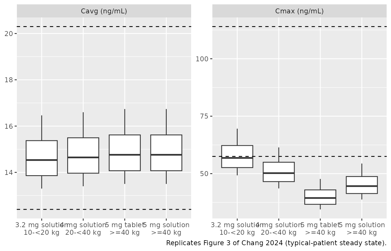
fig3_med <- exp_grid |>
  dplyr::group_by(group) |>
  dplyr::summarise(cavg = median(cavg), cmax = median(cmax), .groups = "drop") |>
  dplyr::mutate(cavg_fig = c(14.5, 14.6, 14.8, 14.8),
                cmax_fig = c(57, 50, 40, 45))
fig3_med |>
  dplyr::rename("Dose group" = group, "Median Cavg, model" = cavg,
                "Median Cmax, model" = cmax, "Median Cavg, Figure 3" = cavg_fig,
                "Median Cmax, Figure 3" = cmax_fig) |>
knitr::kable(digits = 1)| Dose group | Median Cavg, model | Median Cmax, model | Median Cavg, Figure 3 | Median Cmax, Figure 3 |
|---|---|---|---|---|
| 3.2 mg solution | ||||
| 10-<20 kg | 14.5 | 56.8 | 14.5 | 57 |
| 4 mg solution | ||||
| 20-<40 kg | 14.6 | 50.2 | 14.6 | 50 |
| 5 mg tablet | ||||
| >=40 kg | 14.8 | 39.4 | 14.8 | 40 |
| 5 mg solution | ||||
| >=40 kg | 14.8 | 44.6 | 14.8 | 45 |
# Figure medians are read off the box plots to about +/- 0.3 ng/mL (Cavg)
# and +/- 1.5 ng/mL (Cmax).
stopifnot(
  max(abs(fig3_med$cavg / fig3_med$cavg_fig - 1)) < 0.04,
  max(abs(fig3_med$cmax / fig3_med$cmax_fig - 1)) < 0.06
)
As in the paper, Cavg is flat across the bands while Cmax rises as weight falls, because the exponent on V/F (0.54) exceeds that on CL/F (0.31). The highest Cmax, in the 10-<20 kg band, sits at the adult 5 mg twice-daily median.
Replicating Figure 2: individual Cavg on the phase 3 regimen
Figure 2 plots the post hoc Cavg of the phase 3 patients by weight band under the phase 3 dosing (Table S1: 3 mg for 10-<15 kg, 3.5 mg for 15-<25 kg, 4 mg for 25-<40 kg, 5 mg for >= 40 kg). Individual Cavg is dose / (CL/F x tau), so it is driven by the CL/F eta. Weights are drawn uniformly within each band (40-80 kg for the top band), 200 virtual patients per band.
rxode2::rxSetSeed(20240131)
n_per_band <- 200
bands <- data.frame(
  band = c("10-<15 kg", "15-<25 kg", "25-<40 kg", ">=40 kg"),
  lo = c(10, 15, 25, 40), hi = c(15, 25, 40, 80),
  dose = c(3, 3.5, 4, 5), FORM_SOLUTION = c(1L, 1L, 1L, 0L),
  fig2_median = c(14.7, 15.3, 14.4, 14.9)
)
set.seed(20240131)
cohort <- bands[rep(seq_len(nrow(bands)), each = n_per_band), ] |>
  dplyr::mutate(id = dplyr::row_number(),
                weight = stats::runif(dplyr::n(), lo, hi),
                band = factor(band, levels = bands$band))
obs_t <- c(0, 0.25, 0.5, 0.75, 1, 1.5, 2, 3, 4, 6, 8, 10, 12)
ev_cohort <- make_ss_events(cohort, obs_t)
sim_cohort <- rxode2::rxSolve(mod, ev_cohort, returnType = "data.frame") |>
  dplyr::filter(time >= t_last) |>
  dplyr::left_join(dplyr::select(cohort, id, band, dose), by = "id")

cavg_ind <- sim_cohort |>
  dplyr::group_by(id, band, dose) |>
  dplyr::summarise(cl = cl[1], .groups = "drop") |>
  dplyr::mutate(cavg = dose * 1000 / (cl * tau))

ggplot(cavg_ind, aes(band, cavg)) +
  geom_boxplot(outlier.shape = NA) +
  coord_cartesian(ylim = c(5, 40)) +
  labs(x = "Body weight group", y = "Tofacitinib Cavg (ng/mL)",
       caption = "Replicates Figure 2 of Chang 2024 (simulated, 200 per band).")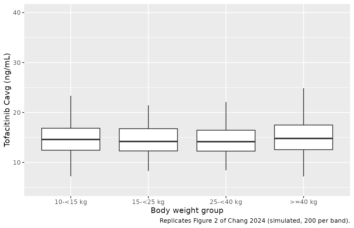
fig2_chk <- cavg_ind |>
  dplyr::group_by(band) |>
  dplyr::summarise(median_cavg = median(cavg),
                   ratio_95_5 = stats::quantile(cavg, 0.95) / stats::quantile(cavg, 0.05),
                   .groups = "drop") |>
  dplyr::left_join(dplyr::select(bands, band, fig2_median), by = "band")
fig2_chk |>
  dplyr::rename("Weight band" = band, "Median Cavg, simulated" = median_cavg,
                "Median Cavg, Figure 2" = fig2_median,
                "95th / 5th percentile" = ratio_95_5) |>
knitr::kable(digits = 2)| Weight band | Median Cavg, simulated | 95th / 5th percentile | Median Cavg, Figure 2 |
|---|---|---|---|
| 10-<15 kg | 14.60 | 2.22 | 14.7 |
| 15-<25 kg | 14.20 | 2.11 | 15.3 |
| 25-<40 kg | 14.16 | 2.21 | 14.4 |
| >=40 kg | 14.80 | 2.15 | 14.9 |
# Centre only: a mis-transcribed CL/F, exponent or dose moves the median by
# tens of percent. Sampling SE of a 200-subject median is about 2%.
stopifnot(max(abs(fig2_chk$median_cavg / fig2_chk$fig2_median - 1)) < 0.12)
The simulated medians sit close to the figure’s, and the 5th-95th percentile spread within each band stays under three-fold, consistent with the paper’s “less than three-fold difference across all individual Cavg values”.
Simulated concentration-time profiles
Steady-state profiles with inter-individual and residual variability for the same cohort (median and 90% prediction interval by band). Figure 1 of the paper is a prediction-corrected VPC against observed data, which is not available here.
vpc <- sim_cohort |>
  dplyr::mutate(tad = time - t_last) |>
  dplyr::group_by(band, tad) |>
  dplyr::summarise(p05 = stats::quantile(sim, 0.05), p50 = stats::median(sim),
                   p95 = stats::quantile(sim, 0.95), .groups = "drop")
ggplot(vpc, aes(tad, p50)) +
  geom_ribbon(aes(ymin = p05, ymax = p95), alpha = 0.25) +
  geom_line() +
  scale_y_log10() +
  facet_wrap(~band) +
  labs(x = "Time after dose (h)", y = "Tofacitinib (ng/mL)",
       caption = "Simulated steady state on the phase 3 regimen; median and 5th-95th percentiles.")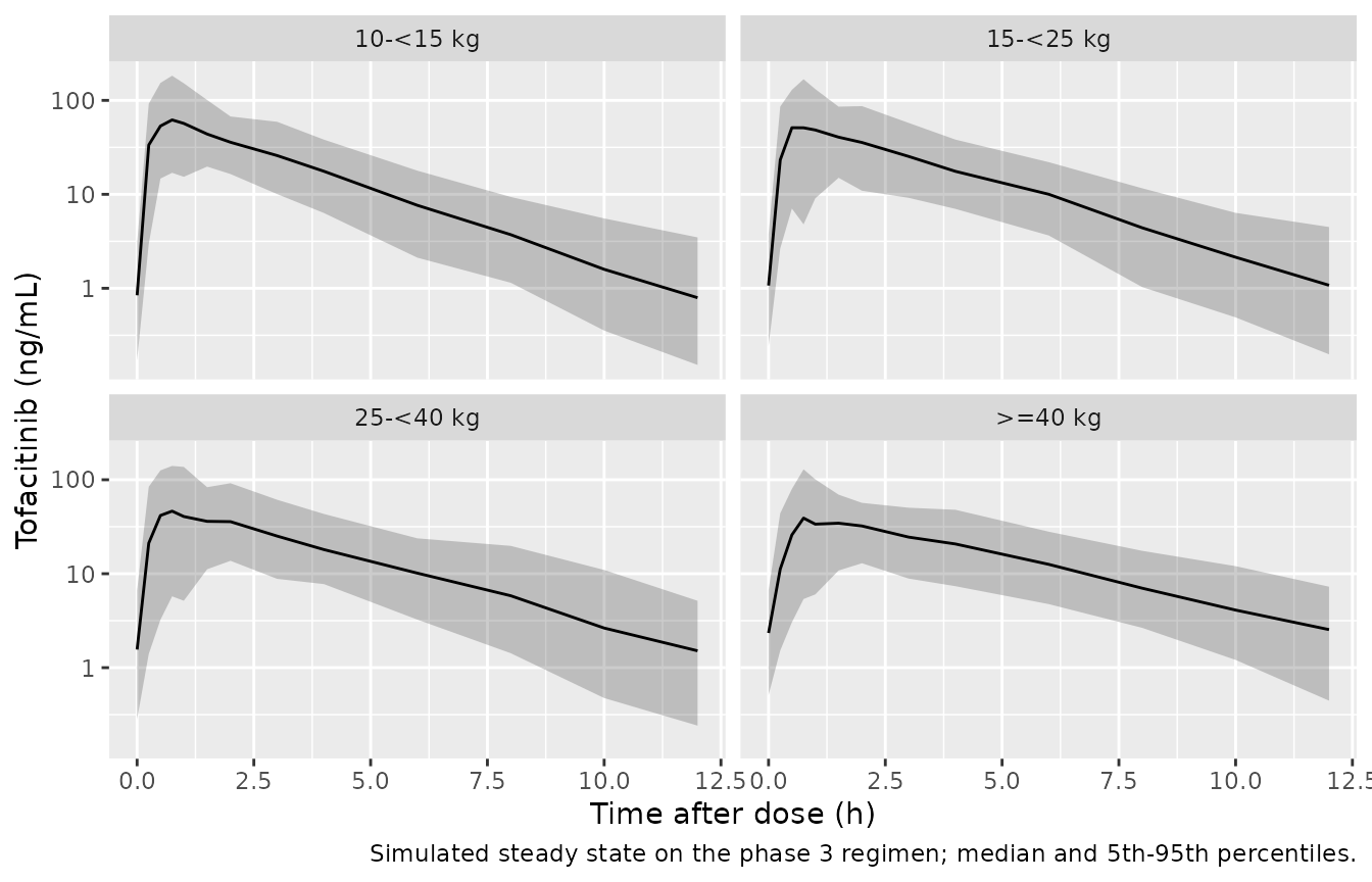
Assumptions and deviations
-
Formulation effect: the Results prose and the control stream
disagree, and the control stream is followed. The Results and
Discussion describe the solution’s ka as “1.64-fold” that of the tablet
(ka ratio 1.64). The control stream sets
KAFORM = (1 + THETA(11))for the solution, and Table 3 lists the rows in$THETAorder, so its “Formulation effect” of 1.64 is THETA(11) itself and the ka ratio is 2.64. Three independent results in the paper confirm the control-stream reading: the solution/tablet Cmax ratio of 113.9% for a typical 46.3 kg patient (1.140 with a ratio of 2.64, 1.079 with 1.64), and every oral-solution Cmax row of Table S5 (within 0.5% with 2.64, 6-7% low with 1.64). -
Table 3 row label. The row “Covariance between CL/F
and V/F” is the scaling factor
SCAL(THETA(6)) that multiplies the CL/F eta in V/F, not an omega element. It is encoded asvc_eta_scale. - IIV variances. Table 3 prints the omega block to two decimals. The CL/F and ka diagonals are taken from the Results-text CVs (23.5% and 120.9%) under CV = sqrt(omega) – the reading under which both round to the Table 3 values (0.06 and 1.46). The off-diagonals and the residual-SD variance are used as printed; the resulting block is positive definite.
-
Residual error is encoded as
lnorm(): the control stream models log-transformed concentrations,Y = LOG(IPRED) + W*EPS(1)with$SIGMA 1 FIX, so the thetas are log-scale SDs. The SD switches at 1.08 h after dose and is scaled per subject byexp(etaruv), an eta that is correlated with the CL/F and ka etas. A commented-out dose-dependent residual term (THETA(8), fixed to 0) is not used by the final model. -
Time-varying weight. The model takes
WTper record. The simulations here hold weight constant within a subject. - Weight distributions for the Figure 2 and Figure 3 replications are uniform within each band, with the open top band capped at 80 kg; the paper does not report the within-band distributions.
- Relative bioavailability study. The healthy-adult crossover (Table 4) was analysed by NCA, not with this model, and is not reproduced; the model’s formulation effect is on ka only, consistent with the AUCinf ratio of 1.04 (90% CI 1.00-1.09) found there.
-
Covariates screened but not retained (age, sex,
race, JIA category, renal and hepatic laboratory values, concomitant
medications, prior DMARD failures) are listed in the model’s
covariatesDataExcludedwhere a canonical column exists.