Petesicatib (Kratochwil 2021)
Source:vignettes/articles/Kratochwil_2021_petesicatib.Rmd
Kratochwil_2021_petesicatib.RmdModel and source
- Citation: Kratochwil NA, Stillhart C, Diack C, Nagel S, Al Kotbi N, Frey N. Population pharmacokinetic analysis of RO5459072, a low water-soluble drug exhibiting complex food-drug interactions. Br J Clin Pharmacol. 2021;87(9):3550-3560. doi:10.1111/bcp.14771
- Description: One-compartment population PK model for oral petesicatib (RO5459072, a cathepsin-S inhibitor) in healthy adults, with dose-dependent proximal-intestine bioavailability, a lagged first-order distal-intestine (colonic) absorption route in the fasted state, and a longer transit chain with dose-independent bioavailability in the fed state
- Article: https://doi.org/10.1111/bcp.14771
Petesicatib (RO5459072, RG7625) is an oral, covalent-reversible inhibitor of cathepsin S that was developed for immune-mediated diseases. It is a poorly water-soluble, highly permeable (BCS class 2) compound. In the first-in-human study it showed a more-than-dose-proportional increase in exposure below 10 mg, a less-than-dose-proportional increase above 30 mg, and an apparent terminal half-life that lengthened with dose, all under fasted conditions; with food these nonlinearities disappeared. Kratochwil 2021 explains all of this with a one-compartment model with linear clearance and a dose-dependent absorption step:
- Fasted, 1 and 3 mg. A depot plus 3 transit compartments feeding the central compartment (the proximal intestine), with a separately estimated bioavailability at each dose.
- Fasted, 10-600 mg. The same proximal chain, with a bioavailability that falls with dose by an Emax function (Equation 1), plus a second, lagged (11.2 h) first-order route from the distal intestine and colon whose bioavailability is the proximal bioavailability times the fraction not absorbed proximally (Equation 2). The late distal input is what lengthens the apparent half-life at high doses.
- Fed. A depot plus 9 transit compartments, dose-independent bioavailability 1.18 relative to fasted 10 mg, and no distal absorption.
The supplement deposits the final NONMEM control stream, which settles the details the article does not print (the shared transit / absorption rate constant, the Hill exponent of 1, the CL-Vc covariance and the log-scale residual error).
Using the model
Each dose must be given twice, once to
depot and once to depot2, exactly as in the
source dataset (NONMEM compartments 1 and 4). The model sets the
bioavailability of each route (f(depot),
f(depot2)) from the DOSE and FED
covariates, so a fed or low-dose record simply puts zero into
depot2. Supply DOSE (mg) and FED
(0/1) on every record.
Population
The analysis used the first-dose PK of two phase 1 studies in healthy male and female volunteers at PRA Health Sciences, Groningen, the Netherlands (Kratochwil 2021 Methods 2.1-2.3 and Results 3.1; supplementary Tables S1-S2):
- the single ascending-dose study NCT02295332 (17 subjects in an interleaved cross-over design; single doses of 1, 3, 10, 30, 100, 300 and 600 mg fasted and 100 mg after a high-fat, high-calorie breakfast), and
- the multiple ascending-dose study NCT02521610 (22 subjects; first doses of 50, 100 or 200 mg given with food, followed from day 3 by twice- or once-daily dosing to day 9).
In total 816 plasma concentrations from 39 subjects entered the model; about 10% were below the 1 ng/mL limit of quantification and were discarded. Each cross-over period of the single-dose study was treated as a separate subject. Neither the article nor its supplement reports age, weight or sex distributions, and no demographic covariate was tested in the model.
The same information is available programmatically via
readModelDb("Kratochwil_2021_petesicatib")()$population.
Source trace
| Element | Value | Source |
|---|---|---|
| CL/F | 9.38 L/h | Table 1; stream THETA(2) |
| Vc/F | 109 L | Table 1; stream THETA(1) |
| kaFaPI, fasted >= 10 mg | 2.05 1/h | Table 1; stream THETA(3), DOSE.GE.10
|
| kaFa (fasted < 10 mg) = kaFe (fed) | 2.95 1/h | Table 1; stream THETA(4) |
| kaFaDI (distal) | 0.065 1/h | Table 1; stream THETA(5) |
| LagFaDI | 11.2 h | Table 1; stream THETA(6) |
| D50 | 216 mg | Table 1; stream THETA(7) |
| Hill exponent | 1 (fixed) | stream THETA(12) 1 FIX; Equation 1 |
| FFaPI, 1 mg / 3 mg | 0.486 / 0.735 | Table 1; stream THETA(9), THETA(10) |
| FFe (fed) | 1.18 | Table 1; stream THETA(11) |
| IIV CL/F, Vc/F (block) | 0.0171, cov 0.0201, 0.0561 | stream $OMEGA BLOCK(2); Table 1 CV 13.1%, 24.0% |
| IIV kaFaPI | 0.108 | stream $OMEGA; Table 1 CV 33.8% |
| IIV kaFe | 0.143 | stream $OMEGA; Table 1 CV 39.2% |
| IIV FFaDI | 0.0979 | stream $OMEGA; Table 1 CV 32.1% |
| IIV D50 | 0.138 | stream $OMEGA; Table 1 CV 38.5% |
| Residual SD (log scale), main | 0.244 | Table 1 (24.4%); stream THETA(8) W1 |
| Residual SD (log scale), fed <= 2 h after first dose | 1.99 | Table 1 (199%); stream THETA(13) W2 |
| Equation 1, FFaPI = 1 - (D-10)/((D-10) + (D50-10)) | Results 3.2 Equation 1; stream TVF1
|
|
| Equation 2, FFaDI = FFaPI (1 - FFaPI) | Results 3.2 Equation 2; stream TVF4
|
|
| Proximal chain: depot + 3 transits (fasted), depot + 9 transits (fed), one rate constant for every step | Figure 2A; stream $DES
|
|
| Distal route: first-order from a lagged, parallel dose compartment | Figure 2A; stream $DES compartment 4,
ALAG4
|
|
| Residual: Y = log(F) + W EPS, SIGMA 1 FIX | stream $ERROR
|
The Table 1 CV% values are reproduced exactly from the stream variances by CV = sqrt(exp(omega^2) - 1) (checked below).
omega <- c(cl = 0.0171, vc = 0.0561, ka_fasted = 0.108, ka_fed = 0.143,
           f_distal = 0.0979, d50 = 0.138)
table1_cv <- c(13.1, 24.0, 33.8, 39.2, 32.1, 38.5)
cv_from_stream <- 100 * sqrt(exp(omega) - 1)
knitr::kable(
  tibble::tibble(Parameter = names(omega), `Stream omega^2` = omega,
                 `CV% from stream` = round(cv_from_stream, 1),
                 `Table 1 CV%` = table1_cv),
  caption = "Stream variances against the Table 1 CV%."
)| Parameter | Stream omega^2 | CV% from stream | Table 1 CV% |
|---|---|---|---|
| cl | 0.0171 | 13.1 | 13.1 |
| vc | 0.0561 | 24.0 | 24.0 |
| ka_fasted | 0.1080 | 33.8 | 33.8 |
| ka_fed | 0.1430 | 39.2 | 39.2 |
| f_distal | 0.0979 | 32.1 | 32.1 |
| d50 | 0.1380 | 38.5 | 38.5 |
Model-derived bioavailability (Figure 2B)
mod <- readModelDb("Kratochwil_2021_petesicatib")
mod_typ <- rxode2::zeroRe(mod)
#> ℹ parameter labels from comments will be replaced by 'label()'
#> Warning: No sigma parameters in the model

# The structure must stay an explicit ODE system (a cl/vc pair must not be
# silently converted to a closed-form linCmt solution).
stopifnot(is.null(rxode2::rxode2(mod)$linCmt))
#> ℹ parameter labels from comments will be replaced by 'label()'

dose_grid <- c(1, 3, seq(10, 600, by = 10))
f_ev <- tibble::tibble(
  id = seq_along(dose_grid), time = 0, amt = 0, evid = 0, cmt = "central",
  DOSE = dose_grid, FED = 0
)
f_ev_fed <- f_ev |> mutate(id = id + length(dose_grid), FED = 1)
f_sim <- rxode2::rxSolve(mod_typ, bind_rows(f_ev, f_ev_fed),
                         returnType = "data.frame", keep = c("DOSE", "FED"))
#> ℹ omega/sigma items treated as zero: 'etalcl', 'etalvc', 'etalka_fastge10', 'etalka_fastlt10fed', 'etalfdepot2', 'etaled50'
#> Warning: multi-subject simulation without without 'omega'
f_tab <- f_sim |>
  transmute(DOSE, FED, FFaPI = f_prox, FFaDI = f_dist, total = f_prox + f_dist)

f_plot <- bind_rows(
  f_tab |> filter(FED == 0) |> select(DOSE, FFaPI, FFaDI, FFa = total) |>
    pivot_longer(-DOSE, names_to = "quantity", values_to = "F"),
  f_tab |> filter(FED == 1, DOSE >= 50, DOSE <= 200) |>
    transmute(DOSE, quantity = "FFe", F = total)
)
ggplot(f_plot, aes(DOSE, F, colour = quantity)) +
  geom_line() +
  geom_point(data = f_plot |> filter(DOSE %in% c(1, 3, 10, 30, 100, 300, 600, 50, 200))) +
  labs(x = "Dose (mg)", y = "Apparent bioavailability (relative to fasted 10 mg)",
       colour = NULL,
       title = "Typical-value apparent bioavailability versus dose",
       caption = "Replicates Figure 2B of Kratochwil 2021 (typical values, no uncertainty bands).")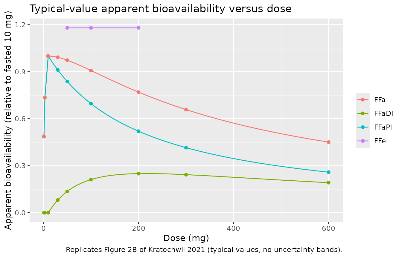
The Results describe this curve numerically; each statement is checked against the packaged model.
fget <- function(dose, col) {
  v <- f_tab[[col]][f_tab$FED == 0 & f_tab$DOSE == dose]
  if (length(v) != 1L) stop("no unique row for dose ", dose)
  v
}
d_fine <- seq(10, 600, by = 1)
ffapi_fine <- 1 - (d_fine - 10) / ((d_fine - 10) + (216 - 10))
ffadi_fine <- ffapi_fine * (1 - ffapi_fine)
claims <- tibble::tribble(
  ~Claim, ~Published, ~Model,
  "FFaPI at 10 mg (reference)", 1, fget(10, "FFaPI"),
  "FFaPI at 600 mg ('decrease with dose from 1 to 0.26')", 0.26, fget(600, "FFaPI"),
  "FFaPI at 1 mg", 0.486, fget(1, "FFaPI"),
  "FFaPI at 3 mg", 0.735, fget(3, "FFaPI"),
  "Maximum FFaDI ('up to 0.25')", 0.25, max(ffadi_fine),
  "Total FFa at 10 mg ('from 1 ...')", 1, fget(10, "total"),
  "Total FFa at 600 mg ('... to 0.5')", 0.5, fget(600, "total"),
  "FFe, fed (dose independent)", 1.18, f_tab$total[f_tab$FED == 1 & f_tab$DOSE == 100]
) |>
  mutate(`% diff` = 100 * (Model - Published) / Published)
knitr::kable(claims, digits = 3,
caption = "Published bioavailability statements against the packaged model.")| Claim | Published | Model | % diff |
|---|---|---|---|
| FFaPI at 10 mg (reference) | 1.000 | 1.000 | 0.000 |
| FFaPI at 600 mg (‘decrease with dose from 1 to 0.26’) | 0.260 | 0.259 | -0.464 |
| FFaPI at 1 mg | 0.486 | 0.486 | 0.000 |
| FFaPI at 3 mg | 0.735 | 0.735 | 0.000 |
| Maximum FFaDI (‘up to 0.25’) | 0.250 | 0.250 | 0.000 |
| Total FFa at 10 mg (‘from 1 …’) | 1.000 | 1.000 | 0.000 |
| Total FFa at 600 mg (‘… to 0.5’) | 0.500 | 0.451 | -9.877 |
| FFe, fed (dose independent) | 1.180 | 1.180 | 0.000 |
# Deterministic evaluations of Equations 1-2. The rounded statements (0.26,
# 0.25, 0.5) carry their own rounding: 0.259 and 0.451 are the exact values.
stopifnot(
  abs(fget(10, "FFaPI") - 1) < 1e-12,
  abs(fget(10, "FFaDI")) < 1e-12,
  abs(fget(600, "FFaPI") - 0.26) < 0.005,
  abs(max(ffadi_fine) - 0.25) < 1e-6,
  abs(d_fine[which.max(ffadi_fine)] - 216) < 1e-9,
  abs(fget(600, "total") - 0.5) < 0.06,
  abs(fget(1, "FFaPI") - 0.486) < 1e-9,
  abs(fget(3, "FFaPI") - 0.735) < 1e-9,
  all(abs(f_tab$total[f_tab$FED == 1] - 1.18) < 1e-9),
  all(f_tab$FFaDI[f_tab$FED == 1] == 0),
  all(f_tab$FFaDI[f_tab$FED == 0 & f_tab$DOSE < 10] == 0)
)
The model places the FFaDI maximum (0.25) at the D50 of 216 mg, where the proximal bioavailability is exactly 0.5; the Results text says FFaDI “increased initially with dose up to 0.25 at around 100 mg”, which reads the maximum off the plotted 100 mg point (FFaDI = 0.21 at 100 mg by Equation 2).
Typical-value mass balance
With linear elimination, the dose-normalised AUC must equal the total bioavailability divided by CL/F for every dose and food state. This checks the dual-compartment dosing, the transit chains and the distal lag together.
arms <- tibble::tribble(
  ~arm,          ~DOSE, ~FED,
  "1 mg fasted",     1,    0,
  "3 mg fasted",     3,    0,
  "10 mg fasted",   10,    0,
  "30 mg fasted",   30,    0,
  "100 mg fasted", 100,    0,
  "300 mg fasted", 300,    0,
  "600 mg fasted", 600,    0,
  "50 mg fed",      50,    1,
  "100 mg fed",    100,    1,
  "200 mg fed",    200,    1
)
arm_levels <- arms$arm

make_events <- function(arms, obs_times, n_per_arm = 1) {
  subj <- arms |>
    slice(rep(seq_len(n()), each = n_per_arm)) |>
    mutate(id = row_number())
  doses <- subj |>
    tidyr::crossing(cmt = c("depot", "depot2")) |>
    mutate(time = 0, amt = DOSE, evid = 1)
  obs <- subj |>
    tidyr::crossing(time = obs_times) |>
    mutate(cmt = "central", amt = 0, evid = 0)
  bind_rows(doses, obs) |>
    select(id, time, amt, evid, cmt, DOSE, FED, arm) |>
    arrange(id, time, desc(evid))
}

dense_times <- sort(unique(c(seq(0, 4, by = 0.02), seq(4, 48, by = 0.1),
                             seq(48, 480, by = 1))))
ev_typ <- make_events(arms, dense_times)
sim_typ <- rxode2::rxSolve(mod_typ, ev_typ, returnType = "data.frame",
                           keep = c("DOSE", "FED", "arm"))
#> ℹ omega/sigma items treated as zero: 'etalcl', 'etalvc', 'etalka_fastge10', 'etalka_fastlt10fed', 'etalfdepot2', 'etaled50'
#> Warning: multi-subject simulation without without 'omega'

conc_typ <- PKNCA::PKNCAconc(sim_typ |> filter(!is.na(Cc)), Cc ~ time | arm + id)
dose_typ <- PKNCA::PKNCAdose(ev_typ |> filter(evid == 1, cmt == "depot"),
                             amt ~ time | arm + id)
int_typ <- data.frame(start = 0, end = Inf, aucinf.obs = TRUE, cmax = TRUE, tmax = TRUE)
nca_typ <- as.data.frame(PKNCA::pk.nca(PKNCA::PKNCAdata(conc_typ, dose_typ, intervals = int_typ)))

f_arm <- sim_typ |>
  group_by(arm) |>
  summarise(F_total = first(f_prox + f_dist), .groups = "drop")
mb <- nca_typ |>
  filter(PPTESTCD == "aucinf.obs") |>
  select(arm, AUCinf = PPORRES) |>
  left_join(arms, by = "arm") |>
  left_join(f_arm, by = "arm") |>
  mutate(expected = F_total * DOSE / 9.38 * 1000,
         `% diff` = 100 * (AUCinf - expected) / expected)
knitr::kable(mb, digits = 3,
caption = "Typical-value AUCinf against F x Dose / (CL/F) (ng*h/mL).")| arm | AUCinf | DOSE | FED | F_total | expected | % diff |
|---|---|---|---|---|---|---|
| 1 mg fasted | 51.812 | 1 | 0 | 0.486 | 51.812 | 0.000 |
| 10 mg fasted | 1066.094 | 10 | 0 | 1.000 | 1066.098 | 0.000 |
| 100 mg fasted | 9675.350 | 100 | 0 | 0.908 | 9675.385 | 0.000 |
| 100 mg fed | 12579.717 | 100 | 1 | 1.180 | 12579.957 | -0.002 |
| 200 mg fed | 25159.432 | 200 | 1 | 1.180 | 25159.915 | -0.002 |
| 3 mg fasted | 235.075 | 3 | 0 | 0.735 | 235.075 | 0.000 |
| 30 mg fasted | 3173.238 | 30 | 0 | 0.992 | 3173.247 | 0.000 |
| 300 mg fasted | 21049.541 | 300 | 0 | 0.658 | 21049.648 | -0.001 |
| 50 mg fed | 6289.859 | 50 | 1 | 1.180 | 6289.979 | -0.002 |
| 600 mg fasted | 28823.734 | 600 | 0 | 0.451 | 28823.899 | -0.001 |
Stochastic simulation (Figure 3)
A virtual cohort of 100 subjects per arm is simulated with the
published interindividual variability, observing at the study sampling
times (0.5-48 h). As in the paper’s VPCs, the early fed residual error
is not applied: the prediction intervals below are of the individual
predictions Cc.
rxode2::rxSetSeed(20210309)
n_per_arm <- 100
study_times <- c(0, 0.5, 1, 2, 3, 4, 5, 6, 8, 10, 12, 24, 36, 48)
ev_cohort <- make_events(arms, study_times, n_per_arm = n_per_arm)
sim <- rxode2::rxSolve(mod, ev_cohort, returnType = "data.frame",
                       keep = c("DOSE", "FED", "arm"))
#> ℹ parameter labels from comments will be replaced by 'label()'
stopifnot(n_distinct(sim$id) == nrow(arms) * n_per_arm)
vpc <- sim |>
  filter(time >= 0.5) |>
  group_by(arm, FED, time) |>
  summarise(p05 = quantile(Cc, 0.05), p50 = median(Cc), p95 = quantile(Cc, 0.95),
            .groups = "drop") |>
  mutate(state = ifelse(FED == 1, "Fed", "Fasted"))
ggplot(vpc |> mutate(arm = factor(arm, levels = arm_levels)),
       aes(time, p50, colour = arm, fill = arm)) +
  geom_ribbon(aes(ymin = p05, ymax = p95), alpha = 0.12, colour = NA) +
  geom_line() +
  facet_wrap(~state) +
  scale_y_log10() +
  labs(x = "Time after dose (h)", y = "Petesicatib concentration (ng/mL)",
       colour = NULL, fill = NULL,
       caption = paste("Replicates Figure 3A-B of Kratochwil 2021:",
                       "median and 90% prediction interval, 100 subjects per arm."))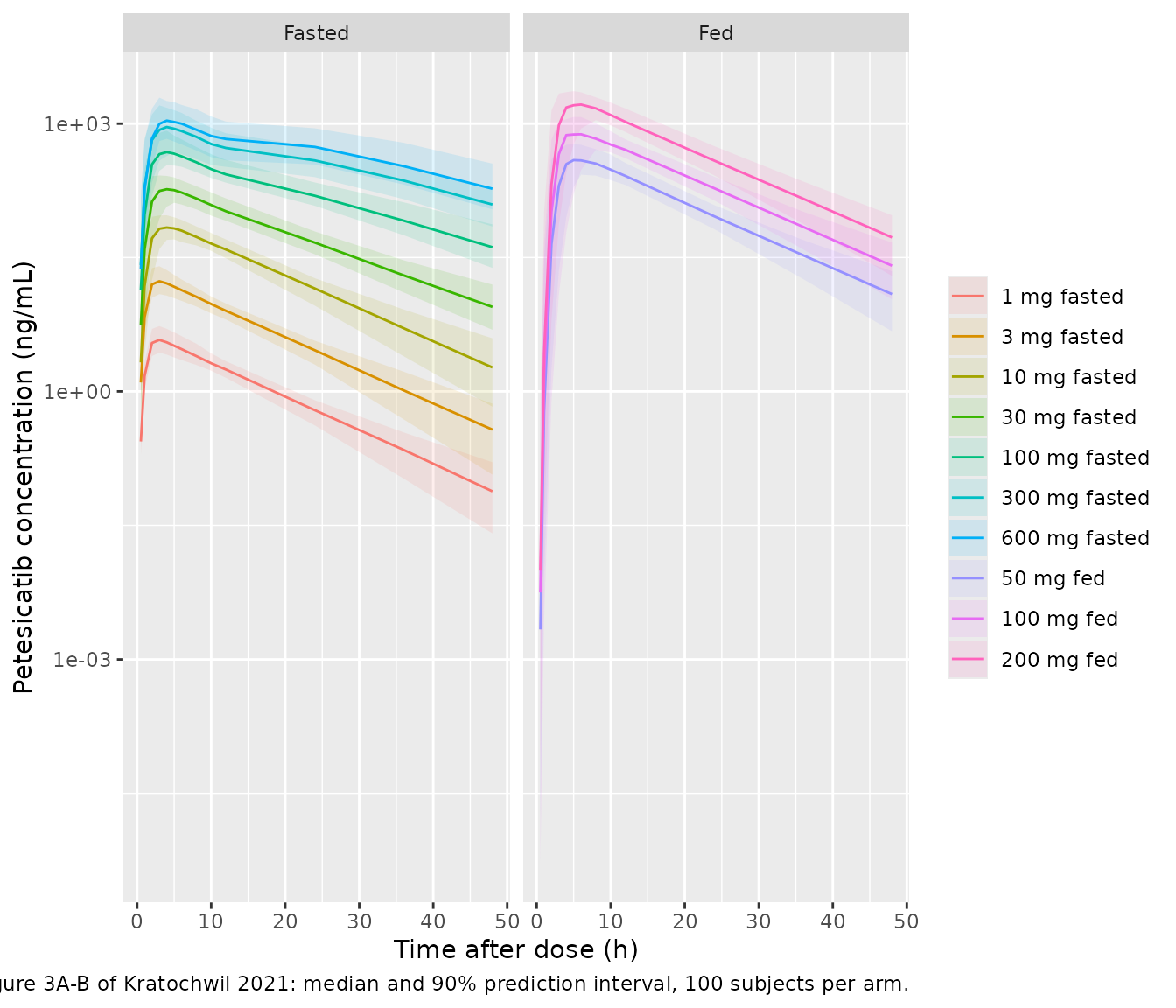
The distal input at 11.2 h is visible as a shoulder in the fasted profiles at 30 mg and above, and it is absent at 1-3 mg and in every fed arm, which is the paper’s explanation of the dose-dependent apparent half-life.
NCA against the published noncompartmental analysis
The simulated concentrations at the study sampling times are analysed with PKNCA, applying the 1 ng/mL LLOQ, and compared with the observed single-dose NCA in supplementary Table S3 (fasted, single ascending dose), Table S4 (100 mg fed, single ascending dose) and Table S5 (day 1 of the multiple ascending dose study; the 50 and 200 mg twice-daily cohorts).
lloq <- 1
nca_input <- sim |>
  select(id, time, Cc, arm) |>
  # Post-dose samples below the 1 ng/mL LLOQ are missing; the time-0
  # pre-dose record is kept.
  mutate(Cc = ifelse(Cc < lloq & time != 0, NA_real_, Cc)) |>
  filter(!is.na(Cc))
conc <- PKNCA::PKNCAconc(nca_input, Cc ~ time | arm + id)
dose <- PKNCA::PKNCAdose(ev_cohort |> filter(evid == 1, cmt == "depot"),
                         amt ~ time | arm + id)
intervals <- data.frame(start = 0, end = Inf, cmax = TRUE, tmax = TRUE,
                        aucinf.obs = TRUE, half.life = TRUE)
nca_res <- PKNCA::pk.nca(PKNCA::PKNCAdata(conc, dose, intervals = intervals))
#> Warning: Too few points for half-life calculation (min.hl.points=3 with only 2
#> points)
nca_df <- as.data.frame(nca_res) |>
  mutate(arm = as.character(arm))
published <- tibble::tribble(
  ~arm,            ~cmax, ~aucinf.obs, ~tmax, ~half.life,
  "1 mg fasted",    4.51,     44.9,    4.00,  5.47,
  "3 mg fasted",    20.8,      229,    5.00,  5.69,
  "10 mg fasted",   81.3,      995,    4.50,  7.89,
  "30 mg fasted",    212,     3240,    4.51,  10.2,
  "100 mg fasted",   516,    10600,    4.00,  13.1,
  "300 mg fasted",  1070,    21000,    3.50,  16.0,
  "600 mg fasted",  1300,    28700,    3.50,  13.3,
  "50 mg fed",       453,     6151,    5.00,  8.29,
  "100 mg fed",      946,    12600,    5.00,  8.8,
  "200 mg fed",     1381,    22294,    4.50,  10.1
)
cmp <- nlmixr2lib::ncaComparisonTable(
  simulated     = nca_df,
  reference     = published,
  by            = "arm",
  params        = c("cmax", "aucinf.obs", "tmax", "half.life"),
  units         = c(cmax = "ng/mL", aucinf.obs = "ng*h/mL", tmax = "h", half.life = "h"),
  tolerance_pct = 20
)
knitr::kable(
  cmp,
  caption = paste("Simulated (median of 100 subjects) vs. published observed NCA",
                  "(geometric mean; Tmax median; N = 4-6 per arm).",
                  "* differs from reference by >20%.")
)| NCA parameter | arm | Reference | Simulated | % diff |
|---|---|---|---|---|
| Cmax (ng/mL) | 1 mg fasted | 4.51 | 3.77 | -16.4% |
| Cmax (ng/mL) | 3 mg fasted | 20.8 | 17.1 | -17.6% |
| Cmax (ng/mL) | 10 mg fasted | 81.3 | 72.4 | -10.9% |
| Cmax (ng/mL) | 30 mg fasted | 212 | 191 | -10.0% |
| Cmax (ng/mL) | 100 mg fasted | 516 | 503 | -2.5% |
| Cmax (ng/mL) | 300 mg fasted | 1070 | 946 | -11.6% |
| Cmax (ng/mL) | 600 mg fasted | 1300 | 1120 | -13.6% |
| Cmax (ng/mL) | 50 mg fed | 453 | 427 | -5.7% |
| Cmax (ng/mL) | 100 mg fed | 946 | 836 | -11.6% |
| Cmax (ng/mL) | 200 mg fed | 1380 | 1760 | +27.1%* |
| Tmax (h) | 1 mg fasted | 4 | 3 | -25.0%* |
| Tmax (h) | 3 mg fasted | 5 | 3 | -40.0%* |
| Tmax (h) | 10 mg fasted | 4.5 | 4 | -11.1% |
| Tmax (h) | 30 mg fasted | 4.51 | 4 | -11.3% |
| Tmax (h) | 100 mg fasted | 4 | 4 | +0.0% |
| Tmax (h) | 300 mg fasted | 3.5 | 4 | +14.3% |
| Tmax (h) | 600 mg fasted | 3.5 | 4 | +14.3% |
| Tmax (h) | 50 mg fed | 5 | 5 | +0.0% |
| Tmax (h) | 100 mg fed | 5 | 5 | +0.0% |
| Tmax (h) | 200 mg fed | 4.5 | 5 | +11.1% |
| AUC0-∞ (obs) (ng*h/mL) | 1 mg fasted | 44.9 | 51.9 | +15.6% |
| AUC0-∞ (obs) (ng*h/mL) | 3 mg fasted | 229 | 235 | +2.5% |
| AUC0-∞ (obs) (ng*h/mL) | 10 mg fasted | 995 | 1090 | +9.5% |
| AUC0-∞ (obs) (ng*h/mL) | 30 mg fasted | 3240 | 3190 | -1.6% |
| AUC0-∞ (obs) (ng*h/mL) | 100 mg fasted | 10600 | 9670 | -8.8% |
| AUC0-∞ (obs) (ng*h/mL) | 300 mg fasted | 21000 | 21700 | +3.4% |
| AUC0-∞ (obs) (ng*h/mL) | 600 mg fasted | 28700 | 30400 | +6.0% |
| AUC0-∞ (obs) (ng*h/mL) | 50 mg fed | 6150 | 6320 | +2.8% |
| AUC0-∞ (obs) (ng*h/mL) | 100 mg fed | 12600 | 12600 | -0.1% |
| AUC0-∞ (obs) (ng*h/mL) | 200 mg fed | 22300 | 25900 | +16.3% |
| t½ (h) | 1 mg fasted | 5.47 | 7.93 | +44.9%* |
| t½ (h) | 3 mg fasted | 5.69 | 8.04 | +41.3%* |
| t½ (h) | 10 mg fasted | 7.89 | 8.19 | +3.8% |
| t½ (h) | 30 mg fasted | 10.2 | 10.2 | -0.1% |
| t½ (h) | 100 mg fasted | 13.1 | 12.6 | -3.5% |
| t½ (h) | 300 mg fasted | 16 | 14.5 | -9.1% |
| t½ (h) | 600 mg fasted | 13.3 | 15.5 | +16.3% |
| t½ (h) | 50 mg fed | 8.29 | 8.24 | -0.6% |
| t½ (h) | 100 mg fed | 8.8 | 8.3 | -5.6% |
| t½ (h) | 200 mg fed | 10.1 | 8.25 | -18.3% |
sim_med <- nca_df |>
  filter(PPTESTCD %in% c("aucinf.obs", "cmax", "half.life")) |>
  group_by(arm, PPTESTCD) |>
  summarise(sim = median(PPORRES, na.rm = TRUE), .groups = "drop")
pub_long <- published |>
  pivot_longer(-arm, names_to = "PPTESTCD", values_to = "pub")
chk <- inner_join(sim_med, pub_long, by = c("arm", "PPTESTCD")) |>
  mutate(pct_diff = 100 * (sim - pub) / pub)
stopifnot(nrow(chk) == 3 * nrow(arms))

auc_chk <- chk |> filter(PPTESTCD == "aucinf.obs")
cmax_chk <- chk |> filter(PPTESTCD == "cmax")
stopifnot(
  # Exposure: a mis-transcribed CL/F, D50, F or unit moves every arm by tens
  # of percent. Centre and a robust envelope, never the extreme arm.
  abs(median(auc_chk$pct_diff)) < 10,
  quantile(abs(auc_chk$pct_diff), 0.9) < 25,
  abs(median(cmax_chk$pct_diff)) < 15,
  quantile(abs(cmax_chk$pct_diff), 0.9) < 30
)

# The distinguishing nonlinearity: the apparent half-life lengthens with dose
# when fasted (distal input) but not when fed.
hl <- chk |> filter(PPTESTCD == "half.life") |> select(arm, sim)
hl_of <- function(a) {
  v <- hl$sim[hl$arm == a]
  if (length(v) != 1L) stop("no unique half-life row for ", a)
  v
}
stopifnot(
  hl_of("300 mg fasted") > 1.3 * hl_of("10 mg fasted"),
  hl_of("100 mg fasted") > 1.2 * hl_of("100 mg fed")
)
Exposure agrees with the observed NCA across the whole 1-600 mg fasted range and the fed arms: AUCinf is within 16% in every arm, and the apparent half-life lengthens with fasted dose (about 8 h at 10 mg to about 15 h at 300-600 mg) while staying near 8 h with food, which is the nonlinearity the model was built to explain. The rows flagged above have identifiable causes:
- Cmax and AUCinf, 200 mg fed. The observed 200 mg cohort had only 4 subjects, and the Discussion notes that their dose-normalised peak concentrations “seemed to be slightly lower than those achieved for doses of 50 and 100 mg”. The model’s fed bioavailability is dose independent, so it predicts proportional exposure at 200 mg.
- Half-life, 1 and 3 mg fasted. The model has one linear clearance, so its shortest possible apparent half-life is the elimination half-life, ln(2) x 109 / 9.38 = 8.1 h. The observed 5.5-5.7 h comes from very low concentrations near the 1 ng/mL LLOQ, a region the paper’s model does not try to describe separately.
- Tmax, 1 and 3 mg fasted. The faster 2.95 1/h chain puts the typical peak at 3 h, on the study grid; the observed medians of 4-5 h come from six subjects each, with ranges of 3-5 h.
Multiple dosing with food (Figure S5)
The paper validated the single-dose model prospectively against the 100 mg once-daily fed cohort of the multiple ascending-dose study (one dose on day 1, then once daily on days 3-9).
md_days <- c(0, 48 + 24 * (0:6))
md_subj <- tibble::tibble(id = 1:100, DOSE = 100, FED = 1)
md_ev <- bind_rows(
  md_subj |> tidyr::crossing(time = md_days, cmt = c("depot", "depot2")) |>
    mutate(amt = DOSE, evid = 1),
  md_subj |> tidyr::crossing(time = seq(0, 216, by = 1)) |>
    mutate(cmt = "central", amt = 0, evid = 0)
) |>
  select(id, time, amt, evid, cmt, DOSE, FED) |>
  arrange(id, time, desc(evid))
md_sim <- rxode2::rxSolve(mod, md_ev, returnType = "data.frame")
md_sum <- md_sim |>
  filter(time >= 0.5) |>
  group_by(time) |>
  summarise(p05 = quantile(Cc, 0.05), p50 = median(Cc), p95 = quantile(Cc, 0.95),
            .groups = "drop")
ggplot(md_sum, aes(time, p50)) +
  geom_ribbon(aes(ymin = p05, ymax = p95), alpha = 0.2) +
  geom_line() +
  labs(x = "Time after first dose (h)", y = "Petesicatib concentration (ng/mL)",
       caption = paste("Replicates Figure S5 of Kratochwil 2021 (100 mg once daily fed):",
                       "median and 90% prediction interval."))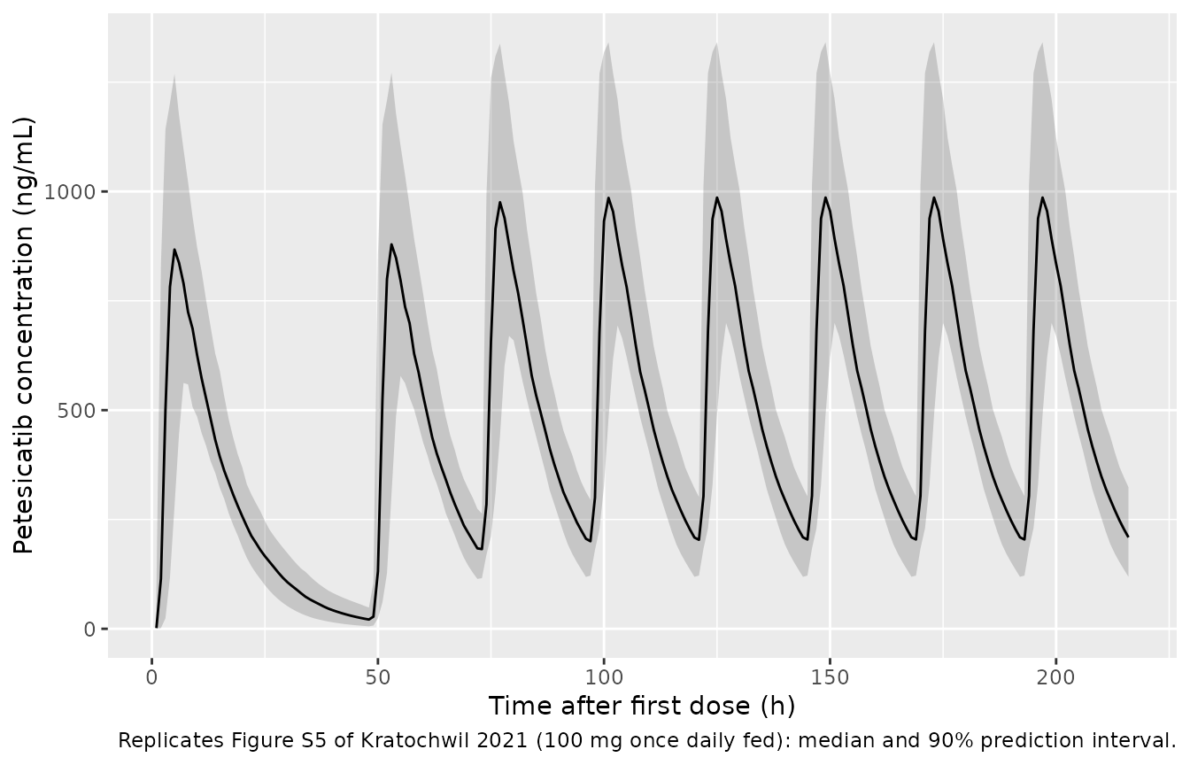
Assumptions and deviations
-
Dose recorded twice. Every dose goes to both
depot(proximal chain, bioavailability FFaPI or FFe) anddepot2(distal route, bioavailability FFaDI, lag 11.2 h), as in the deposited stream, which doses NONMEM compartments 1 and 4 with F1 and F4. -
Transit rate constant. Figure 2A and Table 1 give
only one absorption rate constant per state; the stream’s
$DESuses that same constant for the depot, every transit step and the transfer into the central compartment. The model does the same (no separatektr). -
Fed transit chain. The stream declares 13
compartments while its fed
$DESchain runs throughA(14)and skipsA(11); the chain it implements is depot plus 9 transit compartments, as stated in the Results and drawn in Figure 2A, which is what the model encodes. -
Absorption-rate IIV. Following the stream, the 2.95
1/h rate carries IIV only for fed doses
(
KAF = TVKA3*EXP(ETA(5))); fasted 1 and 3 mg doses use the typical value. The stream also carries an IIV on kaFaDI fixed to a variance of 0, which is omitted here. -
IIV on the distal bioavailability. The stream
applies its FFaDI eta to the derived Equation 2 value
(
F4 = TVF4*EXP(ETA(6))); there is no separate fixed effect, soetalfdepot2has no pairedlfdepot2inini()and the naming checker’s pairing warning is expected. -
CL-Vc covariance. Table 1 lists only the variances;
the covariance (0.0201, correlation 0.65) comes from the stream’s
$OMEGA BLOCK(2). -
Dose-level switches. The stream uses the fasted
Emax branch at
DOSE >= 10mg (Table 1 writes “doses > 3 mg”; no dose between 3 and 10 mg was studied), and defines the low-dose branch only at exactly 1 and 3 mg. The model uses the 1 mg value below 2 mg and the 3 mg value from 2 to 10 mg; doses between 3 and 10 mg are an extrapolation outside the fitted data. -
Food state per subject. The stream switches its
whole
$DESonFOOD, and each cross-over period was analysed as a separate subject, soFEDshould be constant within a simulated subject. -
Residual error. The stream fits log-transformed
concentrations with
Y = log(F) + W*EPS(1)andSIGMA 1 FIX, so the Table 1 “proportional” errors (24.4%, 199%) are log-scale SDs, encoded aslnorm(). The larger SD applies to fed observations within 2 h of the first dose (streamTIME.LE.2.AND.FOOD.EQ.1), taken here astafd() <= 2. -
AUC accumulator. The stream’s auxiliary compartment
CP(cumulative AUC) is not carried; it plays no role in the fitted predictions. - Virtual cohort. No demographic covariates enter the model, so the cohort is defined only by dose, food state and the IIV draws. The simulated NCA uses the study sampling times and the 1 ng/mL LLOQ, but not residual error.