Model and source
- Citation: Mo KH, Chae D, Jung YS, Jin BH, Keum DH, Choi MK, Cha JS, Park MS, Kim CO (2025). Application of population pharmacokinetic modeling of SVG-101 to evaluate proper dose selection. Transl Clin Pharmacol 33(3):156-167. doi:10.12793/tcp.2025.33.e14.
- Description: Two-compartment population PK model for a newly developed dispersible everolimus tablet (SVG-101) in 26 healthy adult Korean males from a randomized, open-label, single-dose, 2x2 crossover bioequivalence study against the reference Afinitor 5 mg tablet (Mo 2025). Only the test (dispersible) arm was used for model development. Absorption is parallel dual-input: fraction Fr_zo = 0.62 of the dose enters the central compartment directly by zero-order input over duration Tk0 = 1.12 h, and the remaining (1 - Fr_zo) = 0.38 enters the intestinal (depot) compartment and is absorbed first-order (ka = 9.48 1/h) after a lag time Tlag = 0.63 h. IIV on all eight structural parameters (log-normal, except the bounded zero-order fraction, which is logit-normal); proportional residual error only. No covariates were retained: age, weight, height, and BMI were screened and none was significant.
- Article (open access): https://doi.org/10.12793/tcp.2025.33.e14
Population
Twenty-six healthy adult Korean males were enrolled in a randomized, open-label, single-dose, 2x2 crossover study at Severance Hospital, Yonsei University Health System (Seoul, Korea). Participants were 19-55 years old by protocol (cohort mean 31.0 years, SD 10.8), weighed at least 55 kg (cohort mean 67.3 kg, SD 8.7), were 171.8 cm tall on average (SD 6.6), and had a body mass index between 18.5 and 27.0 kg/m^2 (cohort mean 22.7, SD 2.3). All were male (Mo 2025 Table 1).
Each participant received a single 5 mg dose of the reference everolimus tablet (Afinitor, Novartis Korea) and a single 5 mg dose of the newly developed dispersible everolimus tablet (SVG-101, test) in the two periods of the crossover, separated by a washout of at least 10 days. Thirteen participants were randomized to the R-T sequence and thirteen to the T-R sequence. Blood was sampled pre-dose and at 0.25, 0.5, 0.75, 1, 1.5, 2, 2.5, 3, 4, 6, 8, 10, 24, 32, 48, 72, 96, 120, and 144 h post-dose.
Only the test (dispersible) occasion contributed to the population PK model: Mo 2025 Methods “Dataset construction for PK analysis” states that “the data pertaining to the R treatment were excised from the dataset because our objective was to develop a PK model for the T treatment.” The model therefore used 842 samples from all 26 subjects, while the non-compartmental analysis in Tables 2 and 3 is based on the 25 subjects who completed both periods. Below-quantification records were left-censored via censoring/limit columns rather than discarded. Estimation was performed in Monolix 2023R1.
The same information is available programmatically via
readModelDb("Mo_2025_everolimus")()$population.
Source trace
The per-parameter origin is recorded as an in-file comment next to
each ini() entry in
inst/modeldb/specificDrugs/Mo_2025_everolimus.R. The table
below collects them in one place for review.
| Equation / parameter | Value | Source location |
|---|---|---|
d/dt(depot) = -ka*depot |
n/a | Mo 2025 p. 161, first displayed equation (dG/dt); Fig. 1 schematic |
d/dt(central) |
n/a | Mo 2025 p. 161, second displayed equation (dAc/dt) |
d/dt(peripheral1) |
n/a | Mo 2025 p. 161, third displayed equation (dAp/dt) |
| Parallel dual absorption (dose split) | n/a | Mo 2025 Fig. 1 caption; Abstract; Results “Model development” |
lka |
9.48 1/h | Table 4, ka, SE 2.99, %RSE 31.6 |
lcl |
7.11 L/h | Table 4, CL, SE 0.40, %RSE 5.6 |
lvc |
47.66 L | Table 4, Vc, SE 2.61, %RSE 5.5 |
lq |
14.32 L/h | Table 4, Q, SE 0.90, %RSE 6.3 |
lvp |
205.94 L | Table 4, Vp, SE 10.89, %RSE 5.3 |
ltk0 |
1.12 h | Table 4, Tk0, SE 0.14, %RSE 12.9 (duration; see Errata 1) |
ltlag |
0.63 h | Table 4, Tlag, SE 0.15, %RSE 24.2 |
logitfr_zo |
logit(0.62) | Table 4, F, SE 0.05, %RSE 8.0 (logit scale; see Errata 2) |
etalka |
0.94^2 = 0.8836 | Table 4, omega_ka, C.V. 118.88% |
etalcl |
0.28^2 = 0.0784 | Table 4, omega_CL, C.V. 28.76% |
etalvc |
0.26^2 = 0.0676 | Table 4, omega_Vc, C.V. 26.66% |
etalq |
0.31^2 = 0.0961 | Table 4, omega_Q, C.V. 31.30% |
etalvp |
0.26^2 = 0.0676 | Table 4, omega_Vp, C.V. 26.38% |
etaltk0 |
0.48^2 = 0.2304 | Table 4, omega_Tk0, C.V. 50.82% |
etaltlag |
0.78^2 = 0.6084 | Table 4, omega_Tlag, C.V. 91.25% |
etalogitfr_zo |
0.76^2 = 0.5776 | Table 4, omega_F, C.V. 27.05% |
propSd |
0.1 | Table 4, sigma_prop, SE 0.0056, %RSE 5.3 |
| Covariate screen (none retained) | n/a | Methods “Population pharmacokinetic modeling”; Results “Model development” |
Proving the random-effect scale
Mo 2025 Table 4 prints omega alongside a
C.V. (%) column, which lets the scale of every random
effect be verified row by row rather than assumed. For a log-normal
random effect, CV = sqrt(exp(omega^2) - 1).
omega_tab <- tibble::tribble(
  ~parameter, ~omega, ~cv_published,
  "ka",   0.94, 118.88,
  "CL",   0.28,  28.76,
  "Vc",   0.26,  26.66,
  "Vp",   0.26,  26.38,
  "Q",    0.31,  31.30,
  "Tk0",  0.48,  50.82,
  "Tlag", 0.78,  91.25,
  "F",    0.76,  27.05
) |>
  mutate(cv_lognormal = 100 * sqrt(exp(omega^2) - 1))

omega_tab |>
  mutate(across(where(is.numeric), \(x) round(x, 2))) |>
  rename(
    "Parameter"            = parameter,
    "omega (Table 4)"      = omega,
    "C.V. % (Table 4)"     = cv_published,
    "C.V. % if log-normal" = cv_lognormal
  ) |>
knitr::kable(caption = "Round-tripping every Table 4 omega through the log-normal CV identity.")| Parameter | omega (Table 4) | C.V. % (Table 4) | C.V. % if log-normal |
|---|---|---|---|
| ka | 0.94 | 118.88 | 119.15 |
| CL | 0.28 | 28.76 | 28.56 |
| Vc | 0.26 | 26.66 | 26.45 |
| Vp | 0.26 | 26.38 | 26.45 |
| Q | 0.31 | 31.30 | 31.76 |
| Tk0 | 0.48 | 50.82 | 50.90 |
| Tlag | 0.78 | 91.25 | 91.51 |
| F | 0.76 | 27.05 | 88.42 |
Seven of the eight rows agree to within rounding of the two-decimal
omega, which confirms that Table 4 reports
omega as the standard deviation of the random effect on its
own transformed scale (so ini() takes
omega^2).
F is the sole exception, and it is a large one: a
log-normal F with omega = 0.76 would have a CV
of 88%, but Table 4 prints 27.05%. Because F is a bounded
proportion, the natural alternative is a logit-normal distribution,
which is also Monolix’s default for such a parameter.
set.seed(1)
n_draw <- 2e5
eta    <- rnorm(n_draw, 0, 0.76)

cv <- function(x) 100 * sd(x) / mean(x)

tibble::tibble(
  Distribution = c("log-normal", "logit-normal", "probit-normal"),
  `Simulated C.V. %` = round(c(
    cv(0.62 * exp(eta)),
    cv(plogis(qlogis(0.62) + eta)),
    cv(pnorm(qnorm(0.62) + eta))
  ), 2),
  `Table 4 C.V. %` = 27.05
) |>
knitr::kable(caption = "Only a logit-normal F reproduces the published C.V. for omega_F.")| Distribution | Simulated C.V. % | Table 4 C.V. % |
|---|---|---|
| log-normal | 88.15 | 27.05 |
| logit-normal | 26.84 | 27.05 |
| probit-normal | 40.05 | 27.05 |
The logit-normal reading reproduces the published 27.05% almost
exactly, so the model file carries F on the logit scale
(logitfr_zo / expit()). This falsifies the
paper’s blanket prose claim that “we assumed a lognormal distribution
for all the model parameters” – see Errata 2.
Virtual cohort
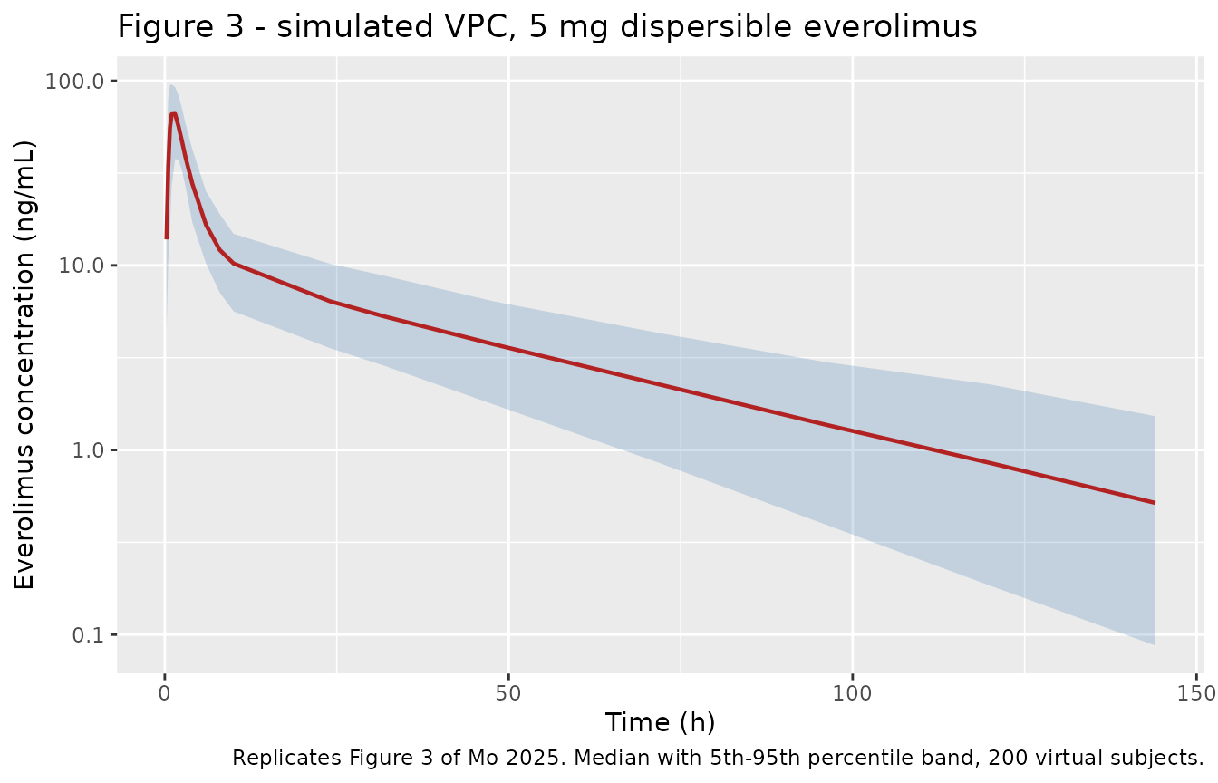
Original observed data are not publicly available. The simulations below use a virtual cohort of 200 subjects receiving the single 5 mg dispersible dose on the published sampling schedule.
Each oral administration is encoded as two parallel dose
records at the same time: one into central
carrying the zero-order arm (with rate = -2 to invoke the
modelled duration dur(central) = Tk0) and one into
depot carrying the first-order arm. Both records carry the
full nominal 5 mg; the model’s f() multipliers split it
into the Fr_zo / (1 - Fr_zo) fractions, so the
pair delivers exactly one dose. Duplicated (id, time, evid)
keys are therefore expected and correct here; the uniqueness guard below
includes cmt, which is the key that must actually be
distinct.
set.seed(20250926)

n_sub    <- 200L
dose_mg  <- 5
obs_grid <- c(0, 0.25, 0.5, 0.75, 1, 1.5, 2, 2.5, 3, 4, 6, 8, 10,
              24, 32, 48, 72, 96, 120, 144)

ids <- seq_len(n_sub)

# First-order arm: dose to depot, ordinary bolus record (alag(depot) = Tlag
# delays it inside the model).
dose_first <- data.frame(
  id = ids, time = 0, amt = dose_mg, evid = 1L,
  cmt = "depot", rate = NA_real_
)

# Zero-order arm: dose to central with rate = -2 so rxode2 uses the modelled
# duration dur(central) = Tk0.
dose_zero <- transform(dose_first, cmt = "central", rate = -2)

obs <- expand.grid(id = ids, time = obs_grid,
                   KEEP.OUT.ATTRS = FALSE, stringsAsFactors = FALSE)
obs$amt  <- NA_real_
obs$evid <- 0L
obs$cmt  <- "central"
obs$rate <- NA_real_

events <- rbind(dose_first, dose_zero, obs[, names(dose_first)])
events$treatment <- "SVG-101 5 mg (test)"

# The two dose records legitimately share (id, time, evid); cmt is what
# distinguishes them, so that is the key the guard has to check.
stopifnot(nrow(dplyr::distinct(events[, c("id", "time", "evid", "cmt")])) == nrow(events))Structural check: which absorption arm carries the lag time?
Mo 2025 reports a single Tlag and describes the model as
“zero-order kinetics, followed by first-order kinetics
with lag time” (Abstract; repeated in the Discussion),
which attaches the lag to the first-order arm. The alternative reading –
lag on the zero-order arm – is simulated here for comparison, on
typical-value (random-effects-zeroed) profiles.
mod_typ <- rxode2::zeroRe(mod)
#> ℹ parameter labels from comments will be replaced by 'label()'

# Alternative reading: move the lag from the depot arm to the central arm.
mod_alt <- mod |>
  rxode2::model(alag(depot) <- 0) |>
  rxode2::model(alag(central) <- tlag, append = TRUE) |>
  rxode2::zeroRe()
#> ℹ parameter labels from comments will be replaced by 'label()'

dense <- c(seq(0, 6, by = 0.01), seq(6.5, 168, by = 0.5))
ev1   <- rbind(
  data.frame(id = 1L, time = 0, amt = dose_mg, evid = 1L, cmt = "depot",   rate = NA_real_),
  data.frame(id = 1L, time = 0, amt = dose_mg, evid = 1L, cmt = "central", rate = -2),
  data.frame(id = 1L, time = dense, amt = NA_real_, evid = 0L, cmt = "central", rate = NA_real_)
)

peak_of <- function(m) {
  s <- rxode2::rxSolve(m, ev1, returnType = "data.frame")
  s[which.max(s$Cc), c("time", "Cc")]
}

pA <- peak_of(mod_typ)
#> ℹ omega/sigma items treated as zero: 'etalka', 'etalcl', 'etalvc', 'etalq', 'etalvp', 'etaltk0', 'etaltlag', 'etalogitfr_zo'
pB <- peak_of(mod_alt)
#> ℹ omega/sigma items treated as zero: 'etalka', 'etalcl', 'etalvc', 'etalq', 'etalvp', 'etaltk0', 'etaltlag', 'etalogitfr_zo'

tibble::tibble(
  Reading = c("A: lag on first-order (depot) arm -- as encoded",
              "B: lag on zero-order (central) arm",
              "Observed (Mo 2025 Table 2, test arm)"),
  `Tmax (h)`      = c(round(pA$time, 2), round(pB$time, 2), 1.50),
  `Cmax (ng/mL)`  = c(round(pA$Cc, 2),   round(pB$Cc, 2),   83.38)
) |>
knitr::kable(caption = "Typical-value Tmax/Cmax under the two lag-time readings. Observed Cmax is the arithmetic mean of Table 2; observed Tmax is the median.")| Reading | Tmax (h) | Cmax (ng/mL) |
|---|---|---|
| A: lag on first-order (depot) arm – as encoded | 1.12 | 84.55 |
| B: lag on zero-order (central) arm | 1.75 | 71.05 |
| Observed (Mo 2025 Table 2, test arm) | 1.50 | 83.38 |
Both readings straddle the observed median Tmax of 1.50 h (reading A
peaks at the end of the zero-order infusion, Tk0 = 1.12 h;
reading B at Tlag + Tk0 = 1.75 h), so Tmax alone does not
settle the question. Cmax does: reading A lands within about 1.5% of the
observed arithmetic mean of 83.38 ng/mL, whereas reading B is roughly
15% low. Together with the unambiguous prose, reading A is adopted in
the model file.
Replicate published figures
# Replicates Figure 3 of Mo 2025: visual predictive check of the final model.
sim |>
  group_by(time) |>
  summarise(
    Q05 = quantile(Cc, 0.05),
    Q50 = quantile(Cc, 0.50),
    Q95 = quantile(Cc, 0.95),
    .groups = "drop"
  ) |>
  filter(time > 0) |>
  ggplot(aes(time, Q50)) +
  geom_ribbon(aes(ymin = Q05, ymax = Q95), alpha = 0.25, fill = "steelblue") +
  geom_line(colour = "firebrick", linewidth = 0.8) +
  scale_y_log10() +
  labs(
    x = "Time (h)", y = "Everolimus concentration (ng/mL)",
    title = "Figure 3 - simulated VPC, 5 mg dispersible everolimus",
    caption = "Replicates Figure 3 of Mo 2025. Median with 5th-95th percentile band, 200 virtual subjects."
  )
The paper’s key clinical result is the steady-state trough simulation of Figure 4, which drives the 3-4 mg daily-dose recommendation. Mo 2025 simulated 1,000 virtual subjects per dose over 200-336 h; this vignette uses 200 per arm over the same window.
# Replicates Figure 4 of Mo 2025: steady-state Ctrough distributions at
# 3, 4, and 5 mg once daily against the 5-15 ng/mL target range.
dose_levels <- c(3, 4, 5)
n_ss        <- 200L
dose_times  <- seq(0, 336 - 24, by = 24)
ss_grid     <- seq(200, 336, by = 1)

make_ss_arm <- function(dose, id_offset) {
  arm_ids <- id_offset + seq_len(n_ss)
  dz <- expand.grid(id = arm_ids, time = dose_times,
                    KEEP.OUT.ATTRS = FALSE, stringsAsFactors = FALSE)
  first_order <- data.frame(dz, amt = dose, evid = 1L, cmt = "depot",   rate = NA_real_)
  zero_order  <- data.frame(dz, amt = dose, evid = 1L, cmt = "central", rate = -2)
  ob <- expand.grid(id = arm_ids, time = ss_grid,
                    KEEP.OUT.ATTRS = FALSE, stringsAsFactors = FALSE)
  ob <- data.frame(ob, amt = NA_real_, evid = 0L, cmt = "central", rate = NA_real_)
  out <- rbind(first_order, zero_order, ob)
  out$dose_group <- paste0(dose, " mg once daily")
  out
}

set.seed(336)
ss_events <- dplyr::bind_rows(
  make_ss_arm(dose_levels[1], id_offset = 0L),
  make_ss_arm(dose_levels[2], id_offset = n_ss),
  make_ss_arm(dose_levels[3], id_offset = 2L * n_ss)
)

ss_sim <- rxode2::rxSolve(mod, events = ss_events, keep = "dose_group",
                          returnType = "data.frame")

ss_sim |>
  filter(time >= 200) |>
  group_by(dose_group, time) |>
  summarise(
    Q05 = quantile(Cc, 0.05),
    Q50 = quantile(Cc, 0.50),
    Q95 = quantile(Cc, 0.95),
    .groups = "drop"
  ) |>
  ggplot(aes(time, Q50)) +
  geom_ribbon(aes(ymin = Q05, ymax = Q95), alpha = 0.25, fill = "steelblue") +
  geom_line(colour = "steelblue", linewidth = 0.7) +
  geom_hline(yintercept = c(5, 15), colour = "firebrick") +
  facet_wrap(~dose_group) +
  labs(
    x = "Time (h)", y = "Everolimus concentration (ng/mL)",
    title = "Figure 4 - steady-state concentrations by once-daily dose",
    caption = "Replicates Figure 4 of Mo 2025. Red lines are the 5-15 ng/mL target trough range."
  )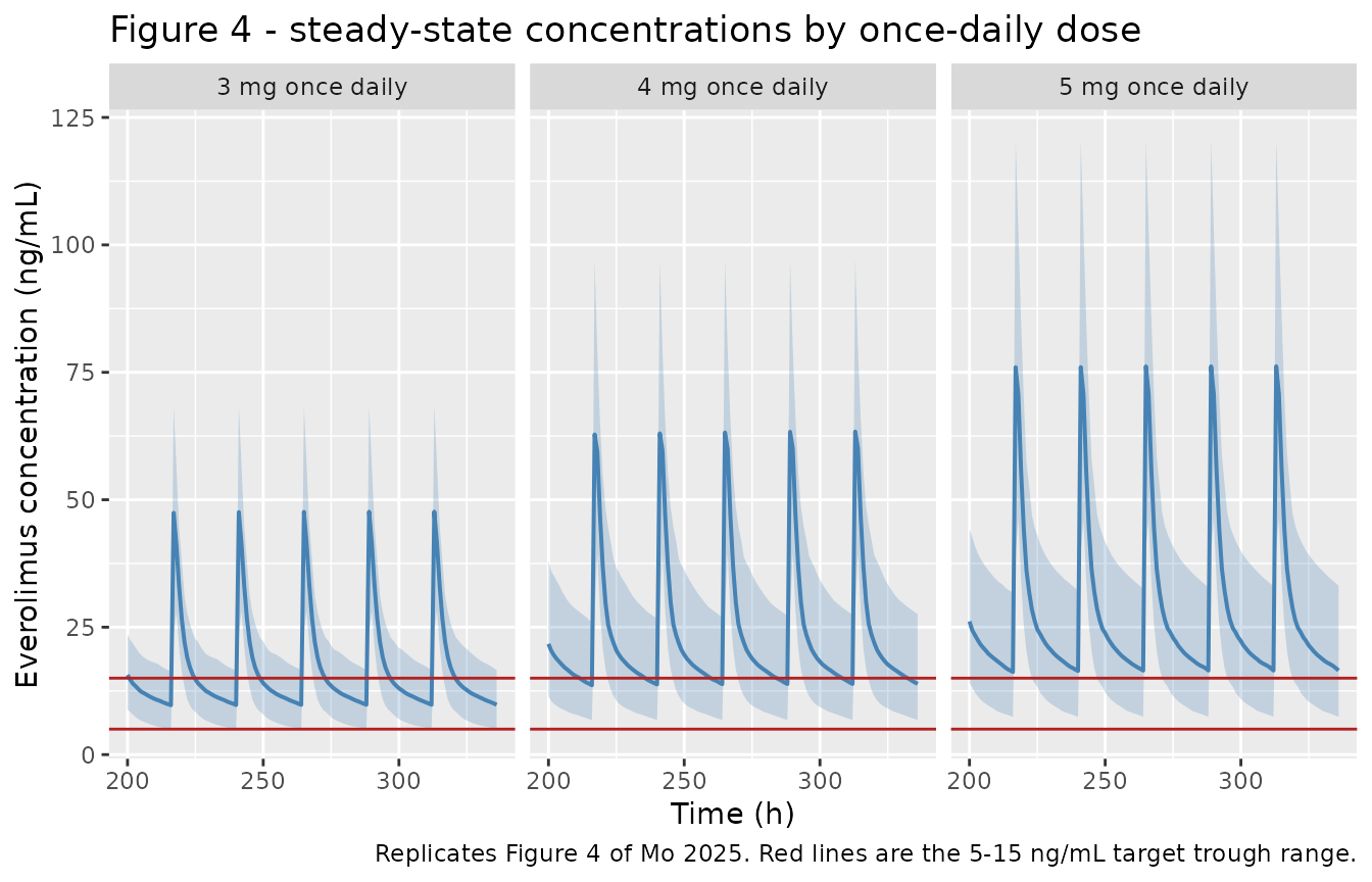
# The paper's dose conclusion is an answer key: 3 mg in range, 4 mg in range
# but elevated, 5 mg above range. Compare the simulated median trough.
trough_times <- seq(216, 336, by = 24)

trough_tab <- ss_sim |>
  filter(time %in% trough_times) |>
  group_by(dose_group) |>
  summarise(
    `5th percentile`  = round(quantile(Cc, 0.05), 2),
    `Median Ctrough`  = round(quantile(Cc, 0.50), 2),
    `95th percentile` = round(quantile(Cc, 0.95), 2),
    .groups = "drop"
  ) |>
  mutate(`Median within 5-15 ng/mL` =
           ifelse(`Median Ctrough` >= 5 & `Median Ctrough` <= 15, "yes", "no")) |>
  rename("Dose group" = dose_group)

knitr::kable(
  trough_tab,
  caption = "Simulated steady-state trough concentrations (ng/mL) vs. the 5-15 ng/mL target."
)| Dose group | 5th percentile | Median Ctrough | 95th percentile | Median within 5-15 ng/mL |
|---|---|---|---|---|
| 3 mg once daily | 5.00 | 9.76 | 16.56 | yes |
| 4 mg once daily | 6.79 | 13.80 | 27.22 | yes |
| 5 mg once daily | 7.40 | 16.48 | 32.45 | no |
This reproduces the paper’s conclusion: the 3 mg and 4 mg median troughs sit inside the 5-15 ng/mL window (with 4 mg noticeably higher), while the 5 mg median exceeds it – exactly the basis for Mo 2025’s recommendation of 3-4 mg daily in this healthy-adult population.
PKNCA validation
sim_nca <- sim |>
  dplyr::filter(!is.na(Cc)) |>
  dplyr::select(id, time, Cc, treatment)

# Guarantee a time = 0 row per subject; pre-dose Cc = 0 is correct for an
# extravascular single dose.
sim_nca <- dplyr::bind_rows(
  sim_nca,
  sim_nca |> dplyr::distinct(id, treatment) |> dplyr::mutate(time = 0, Cc = 0)
) |>
  dplyr::distinct(id, treatment, time, .keep_all = TRUE) |>
  dplyr::arrange(id, treatment, time)

conc_obj <- PKNCA::PKNCAconc(sim_nca, Cc ~ time | treatment + id)

dose_df <- events |>
  dplyr::filter(evid == 1, cmt == "depot") |>
  dplyr::select(id, time, amt, treatment)

dose_obj <- PKNCA::PKNCAdose(dose_df, amt ~ time | treatment + id)

# CL/F and Vz/F are deliberately NOT requested here. PKNCA would form them
# as dose / AUC with the dose in mg and the AUC in h*ng/mL, which yields a
# number 1000x away from L/h and L. Rather than smuggle a scale factor
# through the NCA object, both are reported in the closed-form section
# below, where the mg-to-ng conversion is written out explicitly.
intervals <- data.frame(
  start      = 0,
  end        = Inf,
  cmax       = TRUE,
  tmax       = TRUE,
  auclast    = TRUE,
  aucinf.obs = TRUE,
  half.life  = TRUE
)

nca_res <- PKNCA::pk.nca(PKNCA::PKNCAdata(conc_obj, dose_obj, intervals = intervals))
Comparison against published NCA
Mo 2025 Table 2 reports arithmetic mean (SD) NCA parameters for the test formulation in 25 subjects, except Tmax, which is reported as a median. Table 3 additionally reports the geometric least-squares means for AUCinf (697.90 h*ng/mL) and Cmax (78.87 ng/mL).
published <- tibble::tribble(
  ~treatment,             ~cmax, ~tmax, ~auclast, ~aucinf.obs, ~half.life,
  "SVG-101 5 mg (test)",  83.38, 1.50,  659.38,   723.43,      35.96
)

cmp <- nlmixr2lib::ncaComparisonTable(
  simulated = nca_res,
  reference = published,
  by        = "treatment",
  units     = c(cmax = "ng/mL", tmax = "h", auclast = "h*ng/mL",
                aucinf.obs = "h*ng/mL", half.life = "h"),
  tolerance_pct = 20
)

knitr::kable(
  cmp,
  caption = "Simulated vs. published NCA (Mo 2025 Table 2, test formulation). * differs from reference by >20%."
)| NCA parameter | treatment | Reference | Simulated | % diff |
|---|---|---|---|---|
| Cmax (ng/mL) | SVG-101 5 mg (test) | 83.4 | 75.5 | -9.4% |
| Tmax (h) | SVG-101 5 mg (test) | 1.5 | 1 | -33.3%* |
| AUC0-∞ (obs) (h*ng/mL) | SVG-101 5 mg (test) | 723 | 685 | -5.3% |
| AUClast (h*ng/mL) | SVG-101 5 mg (test) | 659 | 654 | -0.9% |
| t½ (h) | SVG-101 5 mg (test) | 36 | 33.4 | -7.1% |
Cmax, AUClast, AUCinf, and half-life all agree with the published NCA to within 10%, with AUClast within 1%.
Tmax is starred, and the star is an artefact of the sampling
grid rather than a model discrepancy. The simulated median Tmax
is 1.0 h against a published median of 1.5 h – these are adjacent
points on the published sampling schedule (…, 0.75, 1, 1.5, 2, …),
so the smallest resolvable disagreement on that grid is already a 33%
relative difference. The typical-value Tmax is 1.12 h (the end of the
zero-order infusion), which falls between the two sampling times, so
individual subjects round to either side depending on their sampled
Tk0, Tlag, and ka. The comparison
below shows how little separates the two:
tmax_sim <- as.data.frame(nca_res) |>
  dplyr::filter(PPTESTCD == "tmax")

tibble::tibble(
  `Sampling time (h)` = c(0.75, 1.0, 1.5, 2.0, 2.5),
  `Simulated subjects with Tmax here` =
    vapply(c(0.75, 1.0, 1.5, 2.0, 2.5),
           \(t) sum(tmax_sim$PPORRES == t), integer(1))
) |>
knitr::kable(caption = "Distribution of simulated Tmax across the published sampling grid (200 subjects). The published median is 1.5 h; the simulated median is 1.0 h.")| Sampling time (h) | Simulated subjects with Tmax here |
|---|---|
| 0.75 | 37 |
| 1.00 | 64 |
| 1.50 | 55 |
| 2.00 | 24 |
| 2.50 | 9 |
No parameter was adjusted to close this gap.
Closed-form identities
Two disposition quantities can be checked in closed form, independently of the absorption model and of the NCA implementation.
p <- rxode2::rxode(readModelDb("Mo_2025_everolimus"))$theta
#> ℹ parameter labels from comments will be replaced by 'label()'
CL <- exp(p[["lcl"]]); Vc <- exp(p[["lvc"]])
Q  <- exp(p[["lq"]]);  Vp <- exp(p[["lvp"]])

kel <- CL / Vc; k12 <- Q / Vc; k21 <- Q / Vp
b   <- kel + k12 + k21
lambda_z <- (b - sqrt(b^2 - 4 * kel * k21)) / 2

# The 1000 factor converts the 5 mg dose to ng so that Dose / AUC lands in
# L/h against an AUC expressed in h*ng/mL -- the same conversion the model
# applies in `Cc <- 1000 * central / vc`.
tibble::tibble(
  Quantity = c("AUCinf for 5 mg (h*ng/mL)", "Terminal half-life (h)",
               "CL/F (L/h)", "Vz = CL / lambda_z (L)", "Vss = Vc + Vp (L)"),
  Model = round(c(1000 * 5 / CL, log(2) / lambda_z, CL, CL / lambda_z, Vc + Vp), 2),
  Published = c(697.90, 35.96, 7.44, 378.44, NA),
  Source = c("Table 3 GeoLSM AUCinf", "Table 2 t1/2", "Table 2 CL/F",
             "Table 2 Vd/F", "not reported")
) |>
knitr::kable(caption = "Closed-form disposition identities vs. published NCA.")| Quantity | Model | Published | Source |
|---|---|---|---|
| AUCinf for 5 mg (h*ng/mL) | 703.23 | 697.90 | Table 3 GeoLSM AUCinf |
| Terminal half-life (h) | 33.30 | 35.96 | Table 2 t1/2 |
| CL/F (L/h) | 7.11 | 7.44 | Table 2 CL/F |
| Vz = CL / lambda_z (L) | 341.58 | 378.44 | Table 2 Vd/F |
| Vss = Vc + Vp (L) | 253.60 | NA | not reported |
AUCinf = Dose / CL is exact for a linear model and
matches the published geometric least-squares mean to within 1%, which
simultaneously gates the clearance estimate, the mg-to-ng unit
conversion in Cc, and the fact that the two parallel dose
records deliver exactly one dose rather than two.
Assumptions and deviations
-
Whole blood as the observation matrix.
compartmentDatarecordscentralandperipheral1as whole blood. Mo 2025 uses the boilerplate phrase “plasma drug concentration-time curve” in its NCA parameter definitions, but four lines of evidence point to whole blood: samples were drawn into EDTA-K2 tubes and aliquoted with no centrifugation step described (Methods “Study design”); the 5-15 ng/mL target trough range the paper simulates against is the standard whole-blood everolimus therapeutic-drug-monitoring range; the observed concentration magnitudes are whole-blood-scale (everolimus partitions strongly into erythrocytes, so plasma concentrations run several-fold lower); and everolimus monitoring is conventionally whole blood. -
Cohort composition. The virtual cohort carries no
covariates because the final model has none. Age, weight, height, and
BMI were screened by the authors and none was retained; they are
recorded in the model file’s
covariatesDataExcludedfor provenance only. - Cohort size. Figures 3 and 4 use 200 virtual subjects per arm rather than the 1,000 per dose used by Mo 2025 for Figure 4. The published median and percentile bands are stable at this size; the reduction keeps the vignette inside the package’s render-time budget.
- Tmax comparison. The simulated Tmax is read off the published discrete sampling grid, so it is quantized to the same grid the observed median was read from. The typical-value Tmax (1.12 h) falls between the 1 h and 1.5 h sampling times.
- No between-occasion variability. The crossover design would in principle support inter-occasion variability, but only the test occasion entered the model, and Mo 2025 Table 4 reports a single IIV term per parameter with no IOV component.
Errata and deviations from the published text
-
Tk0is a duration, not a rate constant. Mo 2025 Table 4 labelsTk0the “Zero-order absorption rate constant”, but three things contradict that label and agree with each other: the Table 4 row header gives its unit as(h)rather than1/h; the Figure 1 caption definesTk0explicitly as “zero-order absorption duration (h)”; and the symbolTk0is Monolix’s standard name for the duration of a zero-order absorption process. The model file uses the duration reading (dur(central) <- tk0). Under the rate-constant reading the printed unit would be wrong and the absorption phase would last about 0.9 h with no consistent parameterization, so the Table 4 description is treated as the error. -
The zero-order fraction
Fis logit-normal, not log-normal. Mo 2025 Methods states “We assumed a lognormal distribution for all the model parameters”, but Table 4’s ownC.V. (%)column falsifies that forF:omega_F = 0.76yields a log-normal CV of 88.4% against the printed 27.05%, whereas a logit-normalFaboutlogit(0.62)yields 26.8% (a probit-normal yields 39.9%). Every other row round-trips correctly under the log-normal identity. The model file therefore carriesFon the logit scale, which also keeps simulated values inside(0, 1)as a proportion requires. See the “Proving the random-effect scale” section above for the row-by-row check. -
The lag time attaches to the first-order arm. Mo
2025 reports one
Tlagwithout stating which absorption arm it delays. The Abstract and Discussion both phrase the model as “zero-order kinetics, followed by first-order kinetics with lag time”, and the Cmax check in the “Structural check” section above supports that reading over the alternative. The model file usesalag(depot) <- tlag. - Model n = 26 vs. NCA n = 25. The population PK model was fit to all 26 enrolled subjects, while Tables 2 and 3 report NCA on the 25 who completed both crossover periods. One subject withdrew after day 4 but contributed test-formulation data to the model. Comparisons in this vignette are therefore between a 26-subject model and 25-subject NCA summaries.
- Table 3 Cmax point-estimate typo. Mo 2025 Table 3 prints the Cmax geometric mean ratio as “0.6832 (0.6832-0.8604)” – the point estimate erroneously repeats the lower confidence limit. Two independent recomputations give the same corrected value: the GeoLSM columns of the same table yield 78.87 / 102.87 = 0.7667, and the geometric centre of the printed interval is sqrt(0.6832 * 0.8604) = 0.7667. The point estimate should therefore read 0.7667, with the interval (0.6832-0.8604) intact. This value is not used anywhere in the model and is recorded here only for completeness.