Pretomanid (Salinger 2019)
Source:vignettes/articles/Salinger_2019_pretomanid.Rmd
Salinger_2019_pretomanid.Rmd
ui <- rxode2::rxode(readModelDb("Salinger_2019_pretomanid"))
#> ℹ parameter labels from comments will be replaced by 'label()'
#> Warning: some etas defaulted to non-mu referenced, possible parsing error: etae_dose_fdepot, etalmtt, etalfdepot, etaiov_lfdepot_1, etaiov_lcl_1, etaiov_lfdepot_2, etaiov_lcl_2, etaiov_lfdepot_3, etaiov_lcl_3
#> as a work-around try putting the mu-referenced expression on a simple line
Model and source
- Citation: Salinger DH, Subramoney V, Everitt D, Nedelman JR. Population pharmacokinetics of the antituberculosis agent pretomanid. Antimicrob Agents Chemother. 2019;63(10):e00907-19. doi:10.1128/AAC.00907-19
- Description: One-compartment population PK model with three-transit-compartment absorption for pretomanid in healthy subjects and subjects with drug-sensitive, multidrug-resistant or extensively drug-resistant pulmonary tuberculosis
Pretomanid is a nitroimidazooxazine antituberculosis agent. Salinger 2019 pooled 14 studies from the development programme – six phase 1, six phase 2 and two phase 3 – into a single population PK analysis of 17,725 concentrations from 1,054 subjects, spanning healthy volunteers and patients with drug-sensitive (DS), multidrug-resistant (MDR) and extensively drug-resistant (XDR) pulmonary tuberculosis, dosed as monotherapy or in combination regimens for up to 6 months.
The structural model is a one-compartment disposition model
with a three-compartment transit absorption chain feeding a first-order
absorption compartment. At any given dose the model is linear
in both absorption and clearance, but the rate of absorption
and the extent of bioavailability both change with dose. The
chain is (supplemental Table S3 $MODEL, Figure S2):
dose --> transit1 --> transit2 --> transit3 --> depot --> central --> eliminated
           ktr         ktr          ktr          ka        kel
ktr = 3 / MTT, so MTT is the mean transit
time through the three ktr-governed compartments and the
total mean absorption time is MTT + 1/KA – the quantity
Salinger 2019 tabulates in supplemental Table S4. Note that
depot is the source control stream’s ABS
compartment and sits downstream of the transit chain;
oral doses enter transit1, which is why
the model file declares dosing <- "transit1".
cat("ODE states:", paste(ui$state, collapse = " -> "), "\n")
#> ODE states: transit1 -> transit2 -> transit3 -> depot -> central
cat("Observation:", paste(ui$predDf$var, collapse = ", "), "\n")
#> Observation: Cc
cat("Solved-model (linCmt) path used:", ui$props$linCmt, "\n")
#> Solved-model (linCmt) path used: FALSE
# A cl/vc pair can make rxode2 discard explicit ODEs in favour of an analytic
# solution; this model must keep its transit chain, so assert the ODE path.
stopifnot(isFALSE(ui$props$linCmt), length(ui$state) == 5L)
Population
pop <- ui$population
tibble::tibble(Field = names(pop), Value = vapply(pop, function(x) paste(if (!is.null(names(x))) paste0(names(x), " ", x) else x, collapse = "; "), character(1))) |>
knitr::kable(caption = "Population metadata (Salinger 2019 Results 'Data'; Tables S1 and S2).")| Field | Value |
|---|---|
| species | human |
| n_subjects | 1054 |
| n_studies | 14 |
| n_observations | 17725 |
| age_range | 18-77 years |
| age_median | 27 years (healthy subjects), 31 years (subjects with tuberculosis) |
| weight_range | 29-121 kg |
| weight_median | 75 kg (healthy subjects), 53 kg (subjects with tuberculosis) |
| sex_female_pct | 35 |
| race_ethnicity | Black 58.4; Caucasian 14.8; Other 26.8 |
| disease_state | healthy subjects and subjects with drug-sensitive, multidrug-resistant, treatment-intolerant or non-responsive multidrug-resistant, or extensively drug-resistant pulmonary tuberculosis; 24% of subjects with tuberculosis were HIV-positive |
| dose_range | 50-1500 mg single oral dose; 100-1000 mg once daily for 7 days to 6 months |
| regions | North America (all healthy subjects); sub-Saharan Africa (> 95% of subjects with tuberculosis) |
| co_medication | pretomanid given as monotherapy or with bedaquiline, clofazimine, moxifloxacin, linezolid and/or pyrazinamide; antiretrovirals including efavirenz and lopinavir/ritonavir in HIV-positive subjects |
| notes | Six phase 1, six phase 2 and two phase 3 studies (Salinger 2019 Results ‘Data’; per-study detail in Table S1, covariate summary in Table S2). Table S2 tabulates 1056 subjects against the 1054 quoted in Results; the Results figure is used here. Renal function: more than 99% of subjects had normal or only mildly impaired renal function by eGFR. |
Salinger 2019 Table S2 tabulates 1,056 subjects while Results quotes 1,054; the Results figure is carried in the model metadata. All healthy subjects were from North America and none was HIV-positive; more than 95% of the subjects with tuberculosis were from sub-Saharan Africa and 24% of them were HIV-positive.
Source trace
Every fixed-effect and random-effect value in the model file carries
an in-file comment naming its source location. The table below is the
consolidated view. $THETA / $OMEGA /
$SIGMA in the supplemental control file (Table S3) hold
initial estimates only – for example
$THETA 2 is 3.2 against a final 3.30 L/h – so every value
below is taken from Table 1 (final estimates), with
Table S3 supplying the functional form in which each value
enters.
| Quantity | Model parameter | Value | Source |
|---|---|---|---|
| First-order absorption rate constant | lka | 1.38 1/h | Table 1 ‘KA, h-1’ |
| Mean transit time | lmtt | 1.25 h | Table 1 ‘MTT, h’ |
| Clearance, first arm | lcl | 3.30 L/h | Table 1 ‘CL, liters/h’ |
| Clearance, day-5 arm | lcl_late | 3.30 + 0.175 L/h | Table 1 ‘CL’ + ‘SS CL, liters/h’ |
| First clearance breakpoint | ltclchange | 96 h (day 5) | Table S3 SSD conditional |
| Clearance, Nix-TB week-6 arm | lcl_late2 | 3.30 + 0.175 + 0.466 L/h | Table 1 + ‘CL NIX WK >= 6, liters/h’ |
| Second clearance breakpoint | ltclchange2 | 1008 h (week 6) | Table S3 SSWK6 conditional |
| Central volume | lvc | 90.4 L | Table 1 ‘V2, liters’ |
| Relative bioavailability reference | lfdepot | 1 (fixed) | Table 1 ‘F1 (fixed)’ |
| Allometric exponents | e_wt_cl, e_wt_vc | 0.75, 1 (fixed) | Table 1 ‘CL ~ WT’, ‘V2 ~ WT’ |
| Food effect on F1 / KA / MTT | e_fed_fdepot, e_fed_ka, e_fed_mtt | 0.513, 0.482, 0.311 | Table 1 ‘~ FASTED’ rows |
| Dose effects | e_dose_fdepot, e_dose_ka, e_dose_mtt, e_dose_vc | -0.264, -0.128, -0.155, 0.111 | Table 1 ‘~ DOSE’ rows |
| Fed 1000 mg F1 effect | e_dose_1000mg_fdepot | -0.00302 | Table 1 ‘F1 ~ FED&1,000 mg’ |
| Regimen-partner effects | e_moxifloxacin_, e__pyrazinamide_, e_bedaquiline_ | 0.925, 1.25, 0.967, 0.733, 1.32 | Table 1 ‘MOX’, ‘MOX * PZA’, ‘BDQ * MOX * PZA’ rows |
| Antiretroviral effects | e_efv_cl, e_efv_fdepot, e_lpv_cl, e_cyp3a4_ind_cl | 2.17, 1.24, 1.14, 1.35 | Table 1 ‘EFV’, ‘LPVR’, ‘INDUC’ rows |
| HIV effects | e_hiv_pos_cl, e_hiv_pos_fdepot | 0.842, 0.789 | Table 1 ‘CL ~ HIV’, ‘F1 ~ HIV’ |
| Sex effect | e_sexf_cl | 0.837 | Table 1 ‘CL ~ FEMALE’ |
| Disease-state effects | e_dis_healthy_cl, e_dis_tb_mdr_cl, e_dis_tb_mdr_vc, e_dis_tb_xdr_strict_vc | 1.16, 1.15, 1.44, 1.75 | Table 1 ‘HS’, ‘MDR’, ‘XDR’ rows |
| Laboratory effects | e_tbili_fdepot, e_alb_cl | 0.0880, 0.200 | Table 1 ‘TBIL (ref = 5)’, ‘ALB (ref = 35)’ |
| Study effects | e_study_nixtb_fdepot, e_study_nc005_ka, e_study_nc005_mtt | 1.54, 0.186, 6.95e-07 | Table 1 ‘NIX’, ‘NC5’ rows |
| Random-effect modifiers | e_study_nixtb_etalfdepot, e_study_nc003_etalmtt | 0.919, -0.645 | Table 1 ‘F1 Var ~ NIX’, ‘MTT Var ~ NC3’ |
| Box-Cox shapes | boxcox_lcl_, boxcox_lvc_ | 1.36 / 2.78, 9.55 / 26.0 | Table 1 ‘Box-Cox’ rows |
| IIV variances | etalcl, etalvc, etalka + etalmtt + etalfdepot, etae_dose_fdepot | 0.0373, 0.00892, 3x3 block, 0.0274 | Table 1 ‘OMEGA matrix terms’ |
| IOV variances | etaiov_lfdepot_k + etaiov_lcl_k | 0.0412, 0.0101, 0.0185 | Table 1 ‘IOC’ rows; Table S3
$OMEGA BLOCK(2) SAME
|
| Residual error | propSd, powExp, addSd | sqrt(0.548), 0.795, sqrt(11.5) | Table 1 error rows; Table S3 $ERROR
|
Reference subject and covariate scenarios
Salinger 2019 defines a reference subject for its simulations (Results, ‘Model application’): a 55 kg, male, HIV-negative, DS-TB subject with baseline total bilirubin 5 umol/L and albumin 35 g/L, given 200 mg pretomanid once daily, alone, in the fed condition, to steady state.
reference <- list(
  WT = 55, FED = 1, DOSE_PRETOMANID_MG = 200, SEXF = 0, DIS_HEALTHY = 0,
  DIS_TB_MDR = 0, DIS_TB_XDR_STRICT = 0, HIV_POS = 0,
  CONMED_EFV = 0, CONMED_LPV = 0, CONMED_CYP3A4_IND = 0,
  CONMED_MOXIFLOXACIN = 0, CONMED_PYRAZINAMIDE = 0, CONMED_BEDAQUILINE = 0,
  ALB = 35, TBILI = 5,
  STUDY_NC003 = 0, STUDY_NC005 = 0, STUDY_NIXTB = 0,
  OOC1 = 1, OOC2 = 0, OOC3 = 0
)
stopifnot(setequal(names(reference), ui$allCovs))
Typical-value reproduction of the published simulation summary
Supplemental Table S4 summarises simulated steady-state exposure for
23 covariate scenarios. That is the most complete numerical target the
paper offers, so it is the primary gate here. The comparison below is
deterministic: random effects are zeroed with
rxode2::zeroRe(), so each row is the model’s typical-value
prediction for that covariate combination, compared against the paper’s
published median.
Because the random effects on clearance and volume are Box-Cox transformed and strongly right-skewed, a published median is not identical to a typical value – the two differ by a small, reproducible structural offset rather than by simulation noise. The bounds asserted below are therefore tight, but not zero.
tv <- rxode2::zeroRe(ui)
#> Warning: some etas defaulted to non-mu referenced, possible parsing error: etae_dose_fdepot, etalmtt, etalfdepot, etaiov_lfdepot_1, etaiov_lcl_1, etaiov_lfdepot_2, etaiov_lcl_2, etaiov_lfdepot_3, etaiov_lcl_3
#> as a work-around try putting the mu-referenced expression on a simple line

# Solve one covariate scenario to steady state and return both the individual
# parameters and the exposure metrics over the final dosing interval.
solve_scenario <- function(overrides = list(), ndays = 70) {
  cv <- utils::modifyList(reference, overrides)
  tau <- 24
  last_dose <- (ndays - 1) * tau
  ev <- rxode2::et(amt = cv$DOSE_PRETOMANID_MG, cmt = "transit1",
                   ii = tau, until = last_dose) |>
    # Observations sit on the ODE state `central`, never on the algebraic
    # observable `Cc`: naming an observable in `cmt` would auto-inject a
    # compartment slot and renumber the transit chain.
    rxode2::et(seq(last_dose, last_dose + tau, by = 0.25), cmt = "central")
  d <- as.data.frame(ev)
  for (nm in names(cv)) d[[nm]] <- cv[[nm]]
  s <- rxode2::rxSolve(tv, d, returnType = "data.frame",
                       atol = 1e-8, rtol = 1e-8)
  obs <- s[!is.na(s$Cc), ]
  obs$tau <- obs$time - last_dose
  # ug/mL to match the paper's units; the model returns ng/mL.
  cc <- obs$Cc / 1000
  list(
    cl = utils::tail(s$cl, 1), vc = utils::tail(s$vc, 1),
    f1 = utils::tail(s$fdepot, 1), ka = utils::tail(s$ka, 1),
    mtt = utils::tail(s$mtt, 1),
    cavg = sum(diff(obs$tau) * (utils::head(cc, -1) + utils::tail(cc, -1)) / 2) / 24,
    cmax = max(cc), ctau = cc[which.min(abs(obs$tau - 24))],
    tmax = obs$tau[which.max(cc)]
  )
}
scenarios <- tibble::tribble(
  ~scenario,                ~overrides,                                                                      ~cavg, ~ctau, ~cmax, ~thalf, ~clf,  ~vcf,  ~mat,
  "Reference",              list(),                                                                          2.4,   1.6,   3.2,   18,     3.5,   92,    2.1,
  "Fasted",                 list(FED = 0),                                                                   1.2,   0.82,  1.6,   18,     6.8,   180,   2.1,
  "Dose: 100 mg",           list(DOSE_PRETOMANID_MG = 100),                                                  1.2,   0.79,  1.6,   17,     3.5,   86,    2.1,
  "Dose: 400 mg",           list(DOSE_PRETOMANID_MG = 400),                                                  4.7,   3.3,   6.2,   20,     3.6,   100,   2.1,
  "WT: 35 kg",              list(WT = 35),                                                                   3.3,   2.2,   4.6,   17,     2.5,   61,    2.1,
  "WT: 75 kg",              list(WT = 75),                                                                   1.9,   1.3,   2.5,   20,     4.4,   130,   2.1,
  "WT: 100 kg",             list(WT = 100),                                                                  1.5,   1.1,   2.0,   21,     5.4,   170,   2.1,
  "Female",                 list(SEXF = 1),                                                                  2.9,   2.1,   3.7,   22,     2.9,   93,    2.2,
  "Healthy",                list(DIS_HEALTHY = 1),                                                           2.0,   1.3,   2.9,   16,     4.1,   95,    2.1,
  "MDR-TB not in Nix-TB",   list(DIS_TB_MDR = 1),                                                            2.1,   1.5,   2.6,   23,     4.0,   130,   2.1,
  "HIV+",                   list(HIV_POS = 1),                                                               2.2,   1.6,   2.8,   22,     3.8,   120,   2.1,
  "HIV+ & EFV",             list(HIV_POS = 1, CONMED_EFV = 1),                                               1.3,   0.60,  2.1,   10,     6.6,   95,    2.1,
  "HIV+ & LPVr",            list(HIV_POS = 1, CONMED_LPV = 1),                                               1.9,   1.3,   2.5,   19,     4.3,   120,   2.2,
  "Regimen: PaM",           list(CONMED_MOXIFLOXACIN = 1),                                                   2.4,   1.7,   3.2,   19,     3.5,   94,    2.2,
  "Regimen: PaMZ",          list(CONMED_MOXIFLOXACIN = 1, CONMED_PYRAZINAMIDE = 1),                          3.1,   2.4,   3.8,   26,     2.7,   100,   2.2,
  "TBIL: 10 umol/L",        list(TBILI = 10),                                                                2.5,   1.7,   3.4,   18,     3.4,   88,    2.1,
  "ALB: 45 g/L",            list(ALB = 45),                                                                  2.3,   1.5,   3.1,   18,     3.6,   93,    2.2,
  "Dose: 100 mg; fasted",   list(DOSE_PRETOMANID_MG = 100, FED = 0),                                         0.74,  0.48,  0.99,  17,     5.6,   140,   2.0,
  "Extreme low exposure",   list(WT = 100, FED = 0, DIS_TB_MDR = 1, HIV_POS = 1, CONMED_EFV = 1),            0.36,  0.22,  0.50,  15,     23,    480,   2.1,
  "WT: 35 kg; female",      list(WT = 35, SEXF = 1),                                                         4.0,   2.8,   5.2,   20,     2.1,   60,    2.2
)

fitted <- lapply(scenarios$overrides, solve_scenario)
#> ℹ omega/sigma items treated as zero: 'etae_dose_fdepot', 'etalcl', 'etalvc', 'etalka', 'etalmtt', 'etalfdepot', 'etaiov_lfdepot_1', 'etaiov_lcl_1', 'etaiov_lfdepot_2', 'etaiov_lcl_2', 'etaiov_lfdepot_3', 'etaiov_lcl_3'
#> ℹ omega/sigma items treated as zero: 'etae_dose_fdepot', 'etalcl', 'etalvc', 'etalka', 'etalmtt', 'etalfdepot', 'etaiov_lfdepot_1', 'etaiov_lcl_1', 'etaiov_lfdepot_2', 'etaiov_lcl_2', 'etaiov_lfdepot_3', 'etaiov_lcl_3'
#> ℹ omega/sigma items treated as zero: 'etae_dose_fdepot', 'etalcl', 'etalvc', 'etalka', 'etalmtt', 'etalfdepot', 'etaiov_lfdepot_1', 'etaiov_lcl_1', 'etaiov_lfdepot_2', 'etaiov_lcl_2', 'etaiov_lfdepot_3', 'etaiov_lcl_3'
#> ℹ omega/sigma items treated as zero: 'etae_dose_fdepot', 'etalcl', 'etalvc', 'etalka', 'etalmtt', 'etalfdepot', 'etaiov_lfdepot_1', 'etaiov_lcl_1', 'etaiov_lfdepot_2', 'etaiov_lcl_2', 'etaiov_lfdepot_3', 'etaiov_lcl_3'
#> ℹ omega/sigma items treated as zero: 'etae_dose_fdepot', 'etalcl', 'etalvc', 'etalka', 'etalmtt', 'etalfdepot', 'etaiov_lfdepot_1', 'etaiov_lcl_1', 'etaiov_lfdepot_2', 'etaiov_lcl_2', 'etaiov_lfdepot_3', 'etaiov_lcl_3'
#> ℹ omega/sigma items treated as zero: 'etae_dose_fdepot', 'etalcl', 'etalvc', 'etalka', 'etalmtt', 'etalfdepot', 'etaiov_lfdepot_1', 'etaiov_lcl_1', 'etaiov_lfdepot_2', 'etaiov_lcl_2', 'etaiov_lfdepot_3', 'etaiov_lcl_3'
#> ℹ omega/sigma items treated as zero: 'etae_dose_fdepot', 'etalcl', 'etalvc', 'etalka', 'etalmtt', 'etalfdepot', 'etaiov_lfdepot_1', 'etaiov_lcl_1', 'etaiov_lfdepot_2', 'etaiov_lcl_2', 'etaiov_lfdepot_3', 'etaiov_lcl_3'
#> ℹ omega/sigma items treated as zero: 'etae_dose_fdepot', 'etalcl', 'etalvc', 'etalka', 'etalmtt', 'etalfdepot', 'etaiov_lfdepot_1', 'etaiov_lcl_1', 'etaiov_lfdepot_2', 'etaiov_lcl_2', 'etaiov_lfdepot_3', 'etaiov_lcl_3'
#> ℹ omega/sigma items treated as zero: 'etae_dose_fdepot', 'etalcl', 'etalvc', 'etalka', 'etalmtt', 'etalfdepot', 'etaiov_lfdepot_1', 'etaiov_lcl_1', 'etaiov_lfdepot_2', 'etaiov_lcl_2', 'etaiov_lfdepot_3', 'etaiov_lcl_3'
#> ℹ omega/sigma items treated as zero: 'etae_dose_fdepot', 'etalcl', 'etalvc', 'etalka', 'etalmtt', 'etalfdepot', 'etaiov_lfdepot_1', 'etaiov_lcl_1', 'etaiov_lfdepot_2', 'etaiov_lcl_2', 'etaiov_lfdepot_3', 'etaiov_lcl_3'
#> ℹ omega/sigma items treated as zero: 'etae_dose_fdepot', 'etalcl', 'etalvc', 'etalka', 'etalmtt', 'etalfdepot', 'etaiov_lfdepot_1', 'etaiov_lcl_1', 'etaiov_lfdepot_2', 'etaiov_lcl_2', 'etaiov_lfdepot_3', 'etaiov_lcl_3'
#> ℹ omega/sigma items treated as zero: 'etae_dose_fdepot', 'etalcl', 'etalvc', 'etalka', 'etalmtt', 'etalfdepot', 'etaiov_lfdepot_1', 'etaiov_lcl_1', 'etaiov_lfdepot_2', 'etaiov_lcl_2', 'etaiov_lfdepot_3', 'etaiov_lcl_3'
#> ℹ omega/sigma items treated as zero: 'etae_dose_fdepot', 'etalcl', 'etalvc', 'etalka', 'etalmtt', 'etalfdepot', 'etaiov_lfdepot_1', 'etaiov_lcl_1', 'etaiov_lfdepot_2', 'etaiov_lcl_2', 'etaiov_lfdepot_3', 'etaiov_lcl_3'
#> ℹ omega/sigma items treated as zero: 'etae_dose_fdepot', 'etalcl', 'etalvc', 'etalka', 'etalmtt', 'etalfdepot', 'etaiov_lfdepot_1', 'etaiov_lcl_1', 'etaiov_lfdepot_2', 'etaiov_lcl_2', 'etaiov_lfdepot_3', 'etaiov_lcl_3'
#> ℹ omega/sigma items treated as zero: 'etae_dose_fdepot', 'etalcl', 'etalvc', 'etalka', 'etalmtt', 'etalfdepot', 'etaiov_lfdepot_1', 'etaiov_lcl_1', 'etaiov_lfdepot_2', 'etaiov_lcl_2', 'etaiov_lfdepot_3', 'etaiov_lcl_3'
#> ℹ omega/sigma items treated as zero: 'etae_dose_fdepot', 'etalcl', 'etalvc', 'etalka', 'etalmtt', 'etalfdepot', 'etaiov_lfdepot_1', 'etaiov_lcl_1', 'etaiov_lfdepot_2', 'etaiov_lcl_2', 'etaiov_lfdepot_3', 'etaiov_lcl_3'
#> ℹ omega/sigma items treated as zero: 'etae_dose_fdepot', 'etalcl', 'etalvc', 'etalka', 'etalmtt', 'etalfdepot', 'etaiov_lfdepot_1', 'etaiov_lcl_1', 'etaiov_lfdepot_2', 'etaiov_lcl_2', 'etaiov_lfdepot_3', 'etaiov_lcl_3'
#> ℹ omega/sigma items treated as zero: 'etae_dose_fdepot', 'etalcl', 'etalvc', 'etalka', 'etalmtt', 'etalfdepot', 'etaiov_lfdepot_1', 'etaiov_lcl_1', 'etaiov_lfdepot_2', 'etaiov_lcl_2', 'etaiov_lfdepot_3', 'etaiov_lcl_3'
#> ℹ omega/sigma items treated as zero: 'etae_dose_fdepot', 'etalcl', 'etalvc', 'etalka', 'etalmtt', 'etalfdepot', 'etaiov_lfdepot_1', 'etaiov_lcl_1', 'etaiov_lfdepot_2', 'etaiov_lcl_2', 'etaiov_lfdepot_3', 'etaiov_lcl_3'
#> ℹ omega/sigma items treated as zero: 'etae_dose_fdepot', 'etalcl', 'etalvc', 'etalka', 'etalmtt', 'etalfdepot', 'etaiov_lfdepot_1', 'etaiov_lcl_1', 'etaiov_lfdepot_2', 'etaiov_lcl_2', 'etaiov_lfdepot_3', 'etaiov_lcl_3'

pct <- function(sim, pub) 100 * (sim - pub) / pub
compare <- scenarios |>
  mutate(
    cavg_sim  = vapply(fitted, function(x) x$cavg, numeric(1)),
    ctau_sim  = vapply(fitted, function(x) x$ctau, numeric(1)),
    cmax_sim  = vapply(fitted, function(x) x$cmax, numeric(1)),
    thalf_sim = vapply(fitted, function(x) log(2) * x$vc / x$cl, numeric(1)),
    clf_sim   = vapply(fitted, function(x) x$cl / x$f1, numeric(1)),
    vcf_sim   = vapply(fitted, function(x) x$vc / x$f1, numeric(1)),
    mat_sim   = vapply(fitted, function(x) x$mtt + 1 / x$ka, numeric(1)),
    d_cavg = pct(cavg_sim, cavg), d_ctau = pct(ctau_sim, ctau),
    d_cmax = pct(cmax_sim, cmax), d_thalf = pct(thalf_sim, thalf),
    d_clf  = pct(clf_sim, clf),   d_vcf  = pct(vcf_sim, vcf),
    d_mat  = pct(mat_sim, mat)
  )

compare |>
  select(scenario, cavg_sim, cavg, d_cavg, clf_sim, clf, d_clf, thalf_sim, thalf, d_thalf) |>
  rename("Scenario" = scenario, "Cavg,ss sim" = cavg_sim, "Cavg,ss pub" = cavg,
         "% diff" = d_cavg, "CL/F1 sim" = clf_sim, "CL/F1 pub" = clf,
         "% diff " = d_clf, "t1/2 sim" = thalf_sim, "t1/2 pub" = thalf,
         "% diff  " = d_thalf) |>
  knitr::kable(digits = c(0, 3, 2, 1, 3, 2, 1, 1, 0, 1),
caption = "Replicates Table S4 of Salinger 2019: Cavg,ss (ug/mL), apparent oral clearance CL/F1 (L/h) and terminal half-life (h). Simulated values are typical-value predictions; published values are cohort medians.")| Scenario | Cavg,ss sim | Cavg,ss pub | % diff | CL/F1 sim | CL/F1 pub | % diff | t1/2 sim | t1/2 pub | % diff |
|---|---|---|---|---|---|---|---|---|---|
| Reference | 2.398 | 2.40 | -0.1 | 3.475 | 3.5 | -0.7 | 18.0 | 18 | 0.2 |
| Fasted | 1.230 | 1.20 | 2.5 | 6.774 | 6.8 | -0.4 | 18.0 | 18 | 0.2 |
| Dose: 100 mg | 1.199 | 1.20 | -0.1 | 3.475 | 3.5 | -0.7 | 16.7 | 17 | -1.8 |
| Dose: 400 mg | 4.796 | 4.70 | 2.0 | 3.475 | 3.6 | -3.5 | 19.5 | 20 | -2.6 |
| WT: 35 kg | 3.366 | 3.30 | 2.0 | 2.476 | 2.5 | -1.0 | 16.1 | 17 | -5.3 |
| WT: 75 kg | 1.900 | 1.90 | 0.0 | 4.385 | 4.4 | -0.3 | 19.5 | 20 | -2.6 |
| WT: 100 kg | 1.532 | 1.50 | 2.1 | 5.441 | 5.4 | 0.8 | 20.9 | 21 | -0.3 |
| Female | 2.865 | 2.90 | -1.2 | 2.909 | 2.9 | 0.3 | 21.5 | 22 | -2.1 |
| Healthy | 2.067 | 2.00 | 3.4 | 4.031 | 4.1 | -1.7 | 15.5 | 16 | -2.8 |
| MDR-TB not in Nix-TB | 2.085 | 2.10 | -0.7 | 3.996 | 4.0 | -0.1 | 22.6 | 23 | -1.8 |
| HIV+ | 2.247 | 2.20 | 2.1 | 3.708 | 3.8 | -2.4 | 21.4 | 22 | -2.7 |
| HIV+ & EFV | 1.284 | 1.30 | -1.2 | 6.490 | 6.6 | -1.7 | 9.9 | 10 | -1.3 |
| HIV+ & LPVr | 1.971 | 1.90 | 3.7 | 4.228 | 4.3 | -1.7 | 18.8 | 19 | -1.1 |
| Regimen: PaM | 2.480 | 2.40 | 3.3 | 3.360 | 3.5 | -4.0 | 18.6 | 19 | -1.9 |
| Regimen: PaMZ | 3.130 | 3.10 | 1.0 | 2.663 | 2.7 | -1.4 | 25.4 | 26 | -2.2 |
| TBIL: 10 umol/L | 2.549 | 2.50 | 2.0 | 3.269 | 3.4 | -3.8 | 18.0 | 18 | 0.2 |
| ALB: 45 g/L | 2.281 | 2.30 | -0.8 | 3.654 | 3.6 | 1.5 | 17.1 | 18 | -4.7 |
| Dose: 100 mg; fasted | 0.739 | 0.74 | -0.2 | 5.641 | 5.6 | 0.7 | 16.7 | 17 | -1.8 |
| Extreme low exposure | 0.366 | 0.36 | 1.6 | 22.779 | 23.0 | -1.0 | 14.3 | 15 | -4.3 |
| WT: 35 kg; female | 4.021 | 4.00 | 0.5 | 2.072 | 2.1 | -1.3 | 19.2 | 20 | -3.8 |
| Scenario | Cmax,ss sim | Cmax,ss pub | % diff | C24h,ss sim | C24h,ss pub | % diff | V2/F1 sim | V2/F1 pub | % diff | MTT+1/KA sim | MTT+1/KA pub |
|---|---|---|---|---|---|---|---|---|---|---|---|
| Reference | 3.299 | 3.20 | 3.1 | 1.576 | 1.60 | -1.5 | 90.4 | 92 | -1.7 | 1.97 | 2.1 |
| Fasted | 1.630 | 1.60 | 1.9 | 0.807 | 0.82 | -1.6 | 176.2 | 180 | -2.1 | 1.89 | 2.1 |
| Dose: 100 mg | 1.694 | 1.60 | 5.9 | 0.758 | 0.79 | -4.1 | 83.7 | 86 | -2.7 | 1.91 | 2.1 |
| Dose: 400 mg | 6.430 | 6.20 | 3.7 | 3.267 | 3.30 | -1.0 | 97.6 | 100 | -2.4 | 2.04 | 2.1 |
| WT: 35 kg | 4.793 | 4.60 | 4.2 | 2.094 | 2.20 | -4.8 | 57.5 | 61 | -5.7 | 1.97 | 2.1 |
| WT: 75 kg | 2.557 | 2.50 | 2.3 | 1.292 | 1.30 | -0.6 | 123.3 | 130 | -5.2 | 1.97 | 2.1 |
| WT: 100 kg | 2.022 | 2.00 | 1.1 | 1.071 | 1.10 | -2.6 | 164.4 | 170 | -3.3 | 1.97 | 2.1 |
| Female | 3.755 | 3.70 | 1.5 | 2.026 | 2.10 | -3.5 | 90.4 | 93 | -2.8 | 1.97 | 2.2 |
| Healthy | 2.978 | 2.90 | 2.7 | 1.262 | 1.30 | -2.9 | 90.4 | 95 | -4.8 | 1.97 | 2.1 |
| MDR-TB not in Nix-TB | 2.701 | 2.60 | 3.9 | 1.499 | 1.50 | 0.0 | 130.2 | 130 | 0.1 | 1.97 | 2.1 |
| HIV+ | 2.949 | 2.80 | 5.3 | 1.585 | 1.60 | -0.9 | 114.6 | 120 | -4.5 | 1.97 | 2.1 |
| HIV+ & EFV | 2.213 | 2.10 | 5.4 | 0.567 | 0.60 | -5.5 | 92.4 | 95 | -2.7 | 1.97 | 2.1 |
| HIV+ & LPVr | 2.680 | 2.50 | 7.2 | 1.319 | 1.30 | 1.5 | 114.6 | 120 | -4.5 | 1.97 | 2.2 |
| Regimen: PaM | 3.379 | 3.20 | 5.6 | 1.654 | 1.70 | -2.7 | 90.4 | 94 | -3.8 | 1.97 | 2.2 |
| Regimen: PaMZ | 3.944 | 3.80 | 3.8 | 2.340 | 2.40 | -2.5 | 97.7 | 100 | -2.3 | 1.97 | 2.2 |
| TBIL: 10 umol/L | 3.506 | 3.40 | 3.1 | 1.675 | 1.70 | -1.5 | 85.1 | 88 | -3.4 | 1.97 | 2.1 |
| ALB: 45 g/L | 3.185 | 3.10 | 2.7 | 1.464 | 1.50 | -2.4 | 90.4 | 93 | -2.8 | 1.97 | 2.2 |
| Dose: 100 mg; fasted | 1.008 | 0.99 | 1.8 | 0.465 | 0.48 | -3.1 | 135.9 | 140 | -2.9 | 1.81 | 2.0 |
| Extreme low exposure | 0.518 | 0.50 | 3.6 | 0.213 | 0.22 | -3.2 | 471.6 | 480 | -1.8 | 1.89 | 2.1 |
| WT: 35 kg; female | 5.430 | 5.20 | 4.4 | 2.719 | 2.80 | -2.9 | 57.5 | 60 | -4.1 | 1.97 | 2.2 |
# Deterministic typical-value vs published median. A mis-transcribed clearance,
# volume, dose, unit or covariate coefficient moves these by tens of percent;
# the bounds below sit well inside that while admitting the typical-value
# versus median offset created by the Box-Cox random effects.
stopifnot(
  max(abs(compare$d_cavg))  < 10,
  max(abs(compare$d_ctau))  < 12,
  max(abs(compare$d_cmax))  < 12,
  max(abs(compare$d_clf))   < 10,
  max(abs(compare$d_vcf))   < 12,
  max(abs(compare$d_thalf)) < 12,
  max(abs(compare$d_mat))   < 15
)
# Confirm the gate had rows to test (a zero-row comparison would pass vacuously).
stopifnot(nrow(compare) == 20L, !anyNA(compare$d_cavg))
cat("20 scenarios; worst |% difference| across all seven metrics:",
    round(max(abs(c(compare$d_cavg, compare$d_ctau, compare$d_cmax,
                    compare$d_clf, compare$d_vcf, compare$d_thalf,
                    compare$d_mat))), 1), "%\n")
#> 20 scenarios; worst |% difference| across all seven metrics: 10.2 %
The reference row is reproduced by hand arithmetic as well, which pins the units and the day-5 clearance step simultaneously:
The two clearance breakpoints
Salinger 2019 builds clearance as a three-level piecewise-constant
function of time on treatment: an initial arm, a step at study day 5
present in every multiple-dose study, and – for Nix-TB subjects only – a
further step-up at week 6. The supplemental control stream writes this
additively inside one logarithm,
LOG(THETA(2) + SSD*THETA(11) + SSWK6*THETA(38)), so the
model file stores the two later arms as sums and records each published
increment in its source-trace comment.
cv <- utils::modifyList(reference,
  list(DIS_TB_MDR = 1, STUDY_NIXTB = 1, CONMED_BEDAQUILINE = 1))
ev <- rxode2::et(amt = 200, cmt = "transit1", ii = 24, until = 69 * 24) |>
  rxode2::et(c(1, 95, 97, 1007, 1009, 1500), cmt = "central")
d <- as.data.frame(ev)
for (nm in names(cv)) d[[nm]] <- cv[[nm]]
steps <- rxode2::rxSolve(tv, d, returnType = "data.frame")
#> ℹ omega/sigma items treated as zero: 'etae_dose_fdepot', 'etalcl', 'etalvc', 'etalka', 'etalmtt', 'etalfdepot', 'etaiov_lfdepot_1', 'etaiov_lcl_1', 'etaiov_lfdepot_2', 'etaiov_lcl_2', 'etaiov_lfdepot_3', 'etaiov_lcl_3'
steps <- steps[!is.na(steps$Cc), c("time", "cl")]
# Expected arms for this Nix-TB subject: base / day-5 / week-6, each scaled by
# the 1.15-fold drug-resistant-TB effect.
steps$expected <- c(3.30, 3.30, 3.475, 3.475, 3.941, 3.941) * 1.15
steps |>
  rename("Time after first dose (h)" = time, "CL simulated (L/h)" = cl,
         "CL expected (L/h)" = expected) |>
  knitr::kable(digits = c(0, 4, 4),
caption = "Piecewise-constant clearance in a Nix-TB subject. Breakpoints at 96 h (study day 5) and 1008 h (week 6).")| Time after first dose (h) | CL simulated (L/h) | CL expected (L/h) |
|---|---|---|
| 1 | 3.7950 | 3.7950 |
| 95 | 3.7950 | 3.7950 |
| 97 | 3.9963 | 3.9962 |
| 1007 | 3.9963 | 3.9962 |
| 1009 | 4.5322 | 4.5322 |
| 1500 | 4.5322 | 4.5322 |
Study-specific scenarios
Three of Table S4’s rows exercise the study-specific structure: the NC-005 absorption terms, and the Nix-TB bioavailability plus week-6 clearance step. These carry the model’s most extreme Box-Cox shape parameters (26.0 on volume inside Nix-TB), and the paper’s own summary statistics for them are pathological – Table S4 reports a mean half-life of 3.9e+96 h for the TI/NR MDR row – so a published median sits further from the typical value here than in any other row. They are gated separately, with wider bounds and the reason recorded.
study_scen <- tibble::tribble(
  ~scenario, ~overrides, ~cavg, ~cmax, ~clf, ~tmax, ~mat,
  "BPaMZ & MDR-TB & NC-005",
    list(DIS_TB_MDR = 1, STUDY_NC005 = 1, CONMED_BEDAQUILINE = 1,
         CONMED_MOXIFLOXACIN = 1, CONMED_PYRAZINAMIDE = 1), 2.5, 2.9, 3.3, 6.5, 3.8,
  "TI/NR MDR-TB in Nix-TB",
    list(DIS_TB_MDR = 1, STUDY_NIXTB = 1, CONMED_BEDAQUILINE = 1), 2.7, 3.4, 3.0, 4.5, 2.2,
  "XDR-TB in Nix-TB",
    list(DIS_TB_MDR = 1, DIS_TB_XDR_STRICT = 1, STUDY_NIXTB = 1,
         CONMED_BEDAQUILINE = 1), 2.7, 3.3, 3.2, 4.5, 2.2
)
study_fit <- lapply(study_scen$overrides, solve_scenario)
#> ℹ omega/sigma items treated as zero: 'etae_dose_fdepot', 'etalcl', 'etalvc', 'etalka', 'etalmtt', 'etalfdepot', 'etaiov_lfdepot_1', 'etaiov_lcl_1', 'etaiov_lfdepot_2', 'etaiov_lcl_2', 'etaiov_lfdepot_3', 'etaiov_lcl_3'
#> ℹ omega/sigma items treated as zero: 'etae_dose_fdepot', 'etalcl', 'etalvc', 'etalka', 'etalmtt', 'etalfdepot', 'etaiov_lfdepot_1', 'etaiov_lcl_1', 'etaiov_lfdepot_2', 'etaiov_lcl_2', 'etaiov_lfdepot_3', 'etaiov_lcl_3'
#> ℹ omega/sigma items treated as zero: 'etae_dose_fdepot', 'etalcl', 'etalvc', 'etalka', 'etalmtt', 'etalfdepot', 'etaiov_lfdepot_1', 'etaiov_lcl_1', 'etaiov_lfdepot_2', 'etaiov_lcl_2', 'etaiov_lfdepot_3', 'etaiov_lcl_3'
study_cmp <- study_scen |>
  mutate(
    cavg_sim = vapply(study_fit, function(x) x$cavg, numeric(1)),
    cmax_sim = vapply(study_fit, function(x) x$cmax, numeric(1)),
    clf_sim  = vapply(study_fit, function(x) x$cl / x$f1, numeric(1)),
    tmax_sim = vapply(study_fit, function(x) x$tmax, numeric(1)),
    mat_sim  = vapply(study_fit, function(x) x$mtt + 1 / x$ka, numeric(1))
  )
study_cmp |>
  select(scenario, cavg_sim, cavg, cmax_sim, cmax, clf_sim, clf, tmax_sim, tmax, mat_sim, mat) |>
  rename("Scenario" = scenario, "Cavg,ss sim" = cavg_sim, "Cavg,ss pub" = cavg,
         "Cmax,ss sim" = cmax_sim, "Cmax,ss pub" = cmax, "CL/F1 sim" = clf_sim,
         "CL/F1 pub" = clf, "Tmax sim" = tmax_sim, "Tmax pub" = tmax,
         "MTT+1/KA sim" = mat_sim, "MTT+1/KA pub" = mat) |>
  knitr::kable(digits = c(0, 3, 2, 3, 2, 3, 2, 2, 1, 2, 1),
caption = "Replicates the three study-specific rows of Table S4 (Salinger 2019). Tmax and MTT + 1/KA are in h, concentrations in ug/mL, CL/F1 in L/h.")| Scenario | Cavg,ss sim | Cavg,ss pub | Cmax,ss sim | Cmax,ss pub | CL/F1 sim | CL/F1 pub | Tmax sim | Tmax pub | MTT+1/KA sim | MTT+1/KA pub |
|---|---|---|---|---|---|---|---|---|---|---|
| BPaMZ & MDR-TB & NC-005 | 2.577 | 2.5 | 2.954 | 2.9 | 3.234 | 3.3 | 6.5 | 6.5 | 3.90 | 3.8 |
| TI/NR MDR-TB in Nix-TB | 2.832 | 2.7 | 3.788 | 3.4 | 2.943 | 3.0 | 4.0 | 4.5 | 1.97 | 2.2 |
| XDR-TB in Nix-TB | 2.832 | 2.7 | 3.609 | 3.3 | 2.943 | 3.2 | 4.0 | 4.5 | 1.97 | 2.2 |
stopifnot(
  max(abs(pct(study_cmp$cavg_sim, study_cmp$cavg))) < 12,
  max(abs(pct(study_cmp$cmax_sim, study_cmp$cmax))) < 18,
  max(abs(pct(study_cmp$clf_sim,  study_cmp$clf)))  < 12,
  max(abs(pct(study_cmp$mat_sim,  study_cmp$mat)))  < 12
)
The NC-005 row is the sharpest single confirmation that the absorption model has been transcribed correctly. Salinger 2019 Results (‘Tmax’) reports that median Tmax was 4.25 h under reference conditions and varied by only +/- 0.25 h in every examined condition except study NC-005, where it was 6.5 h – an anomaly the authors called “suspected to be spurious” but could not reject because the study had no samples between 4 and 8 h post-dose. The model reproduces that value:
nc005 <- study_cmp[study_cmp$scenario == "BPaMZ & MDR-TB & NC-005", ]
stopifnot(nrow(nc005) == 1L)
ref_tmax <- solve_scenario()$tmax
#> ℹ omega/sigma items treated as zero: 'etae_dose_fdepot', 'etalcl', 'etalvc', 'etalka', 'etalmtt', 'etalfdepot', 'etaiov_lfdepot_1', 'etaiov_lcl_1', 'etaiov_lfdepot_2', 'etaiov_lcl_2', 'etaiov_lfdepot_3', 'etaiov_lcl_3'
cat("NC-005 simulated steady-state Tmax:", nc005$tmax_sim, "h (published 6.5 h)\n")
#> NC-005 simulated steady-state Tmax: 6.5 h (published 6.5 h)
cat("Reference simulated steady-state Tmax:", ref_tmax, "h (published 4.25 h)\n")
#> Reference simulated steady-state Tmax: 4 h (published 4.25 h)
# Both are read off the same quarter-hour grid the paper used, so a quarter-hour
# tolerance is the resolution of the comparison itself.
stopifnot(abs(nc005$tmax_sim - 6.5) <= 0.25, abs(ref_tmax - 4.25) <= 0.5)
That late peak comes entirely from the NC-005 absorption
rate effect (e_study_nc005_ka = 0.186, giving
KA = 0.257 1/h and 1/KA = 3.9 h), not from the
transit chain – see the Errata below on the MTT ~ NC5
boundary estimate.
Virtual cohort and steady-state NCA
The cohort below is 200 reference subjects, the per-arm cap for validation vignettes. Random effects are drawn by rxode2, including the interoccasion effects on bioavailability and clearance for occasion 1.
# rxSetSeed()/set.seed() cannot make this cohort identical across machines:
# rxode2 partitions its RNG streams per solver thread, so a 2-core CI runner
# and a 16-thread workstation draw different cohorts from identical source.
# Every assertion below is therefore written on the centre of the distribution
# or on robust quantiles -- never on an extreme, a sign, or an exact zero.
rxode2::rxSetSeed(20190923)
n_sub <- 200L
tau <- 24
ndays <- 28
last_dose <- (ndays - 1) * tau
dose_ev <- rxode2::et(amt = 200, cmt = "transit1", ii = tau, until = last_dose)
# Sparse sampling while accumulation completes, dense sampling over the final
# dosing interval so Cmax / Tmax / AUC are resolved. A grid too coarse around
# Tmax understates AUC by several percent.
obs_times <- sort(unique(c(seq(0, last_dose, by = 6),
                           seq(last_dose, last_dose + tau, by = 0.25))))
ev1 <- as.data.frame(rxode2::et(dose_ev) |> rxode2::et(obs_times, cmt = "central"))
# Replicate the schedule across subjects explicitly. `nSub` is ignored when the
# event table already carries an `id` column, which `as.data.frame(et(...))`
# always adds, so the cohort would silently collapse to one subject.
ev1$id <- NULL
events <- ev1[rep(seq_len(nrow(ev1)), times = n_sub), , drop = FALSE]
events$id <- rep(seq_len(n_sub), each = nrow(ev1))
for (nm in names(reference)) events[[nm]] <- reference[[nm]]
events$treatment <- "200 mg q.d. fed"
events <- events[order(events$id, events$time), ]

sim <- rxode2::rxSolve(ui, events, keep = "treatment",
                       returnType = "data.frame")
if (is.null(sim$id)) sim$id <- 1L
cat("simulated rows:", nrow(sim), "subjects:", dplyr::n_distinct(sim$id), "\n")
#> simulated rows: 41000 subjects: 200
stopifnot(dplyr::n_distinct(sim$id) == n_sub, all(sim$Cc[!is.na(sim$Cc)] >= 0))
ss <- sim |>
  filter(!is.na(Cc), time >= last_dose) |>
  mutate(tad = time - last_dose, conc = Cc / 1000)
bands <- ss |>
  group_by(tad) |>
  summarise(p05 = quantile(conc, 0.05), p50 = median(conc),
            p95 = quantile(conc, 0.95), .groups = "drop")
ggplot(bands, aes(x = tad)) +
  geom_ribbon(aes(ymin = p05, ymax = p95), alpha = 0.25, fill = "steelblue") +
  geom_line(aes(y = p50), linewidth = 0.9, colour = "steelblue4") +
  labs(x = "Time after dose at steady state (h)",
       y = "Pretomanid concentration (ug/mL)",
       title = "Steady-state profile, 200 mg q.d. fed, reference covariates",
       subtitle = "Median with 5th-95th percentile band; 200 simulated subjects") +
  theme_bw()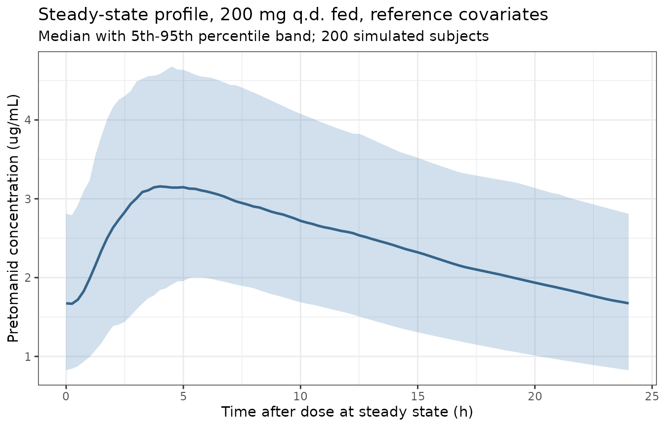
In the spirit of Figure 1 of Salinger 2019 (prediction-corrected visual predictive checks) this shows the median and the 5th-95th percentile envelope; it is an illustrative steady-state envelope rather than a reproduction of the paper’s pcVPC, which requires the original observations.
# PKNCA input filter is `!is.na(Cc)` ONLY -- adding `time > 0` or `Cc > 0`
# would drop the time-zero anchor and trigger the "AUC range starting before
# the first measurement" warning for every subject.
conc_df <- sim |>
  filter(!is.na(Cc)) |>
  transmute(id, time, Cc = Cc / 1000, treatment)
# Guarantee a time-zero row per subject; pre-dose Cc = 0 is correct for an
# extravascular dose.
conc_df <- conc_df |>
  bind_rows(conc_df |> distinct(id, treatment) |> mutate(time = 0, Cc = 0)) |>
  distinct(id, treatment, time, .keep_all = TRUE) |>
  arrange(id, time)

dose_df <- events |>
  filter(evid == 1) |>
  select(id, time, amt, treatment)
stopifnot(dplyr::n_distinct(dose_df$id) == n_sub)

conc_obj <- PKNCA::PKNCAconc(conc_df, Cc ~ time | treatment + id,
                             concu = "ug/mL", timeu = "h")
dose_obj <- PKNCA::PKNCAdose(dose_df, amt ~ time | treatment + id,
                             doseu = "mg")
intervals <- data.frame(
  start = last_dose, end = last_dose + tau,
  cmax = TRUE, tmax = TRUE, cav = TRUE, auclast = TRUE
)
nca <- PKNCA::pk.nca(PKNCA::PKNCAdata(conc_obj, dose_obj, intervals = intervals))
nca_res <- as.data.frame(nca)
stopifnot(nrow(nca_res) > 0)
Comparison against the published simulation summary
Table S4’s Reference row reports the median, 10th and 90th
percentiles across the paper’s simulated cohort. The cohort statistics
below are compared against it; tmax is reported on the
paper’s quarter-hour grid.
per_sub <- nca_res |>
  filter(PPTESTCD %in% c("cmax", "tmax", "cav")) |>
  select(id, PPTESTCD, PPORRES) |>
  tidyr::pivot_wider(names_from = PPTESTCD, values_from = PPORRES)

# C24h,ss is read straight off the dense grid at exactly 24 h after the final
# dose. PKNCA's `ctrough` is anchored differently and returns NA for this
# interval, and the trough needs no interpolation here because the simulation
# grid lands on the interval end exactly.
c24h <- sim |>
  filter(!is.na(Cc), time == last_dose + tau) |>
  transmute(id, ctau = Cc / 1000)
stopifnot(nrow(c24h) == n_sub)
per_sub <- left_join(per_sub, c24h, by = "id")
stopifnot(nrow(per_sub) == n_sub,
          !anyNA(per_sub$cav), !anyNA(per_sub$cmax),
          !anyNA(per_sub$tmax), !anyNA(per_sub$ctau))

published_ref <- tibble::tribble(
  ~metric, ~median_pub, ~p10_pub, ~p90_pub,
  "Cavg,ss (ug/mL)", 2.4, 1.6,  3.5,
  "Cmax,ss (ug/mL)", 3.2, 2.2,  4.6,
  "C24h,ss (ug/mL)", 1.6, 0.93, 2.6,
  "Tmax,ss (h)",     4.2, 2.8,  7.2
)
sim_stats <- tibble::tibble(
  metric = published_ref$metric,
  median_sim = c(median(per_sub$cav), median(per_sub$cmax),
                 median(per_sub$ctau), median(per_sub$tmax)),
  p10_sim = c(quantile(per_sub$cav, 0.10), quantile(per_sub$cmax, 0.10),
              quantile(per_sub$ctau, 0.10), quantile(per_sub$tmax, 0.10)),
  p90_sim = c(quantile(per_sub$cav, 0.90), quantile(per_sub$cmax, 0.90),
              quantile(per_sub$ctau, 0.90), quantile(per_sub$tmax, 0.90))
)
ref_cmp <- published_ref |>
  left_join(sim_stats, by = "metric") |>
  mutate(pct_median = pct(median_sim, median_pub))
ref_cmp |>
  select(metric, median_sim, median_pub, pct_median, p10_sim, p10_pub, p90_sim, p90_pub) |>
  rename("Metric" = metric, "Median sim" = median_sim, "Median pub" = median_pub,
         "% diff (median)" = pct_median, "10th sim" = p10_sim, "10th pub" = p10_pub,
         "90th sim" = p90_sim, "90th pub" = p90_pub) |>
  knitr::kable(digits = c(0, 3, 2, 1, 3, 2, 3, 2),
caption = "Replicates the Reference row of Table S4 (Salinger 2019) from a 200-subject simulated cohort.")| Metric | Median sim | Median pub | % diff (median) | 10th sim | 10th pub | 90th sim | 90th pub |
|---|---|---|---|---|---|---|---|
| Cavg,ss (ug/mL) | 2.454 | 2.4 | 2.2 | 1.577 | 1.60 | 3.428 | 3.5 |
| Cmax,ss (ug/mL) | 3.244 | 3.2 | 1.4 | 2.209 | 2.20 | 4.538 | 4.6 |
| C24h,ss (ug/mL) | 1.674 | 1.6 | 4.6 | 0.949 | 0.93 | 2.493 | 2.6 |
| Tmax,ss (h) | 4.250 | 4.2 | 1.2 | 2.750 | 2.80 | 7.025 | 7.2 |
# Assertions on the CENTRE of a simulated cohort, which is stable across
# cohorts and thread counts. A mis-transcribed dose, clearance, volume or unit
# moves the median by tens of percent.
stopifnot(all(abs(ref_cmp$pct_median) < 20))
# Spread: the paper's Reference row reports a 32% CV on Cavg,ss. Assert the
# ORDER of magnitude of the spread rather than a tight bound, because it is
# unclear from the paper whether its simulation carried the interoccasion
# random effects that this model draws.
cv_cavg <- 100 * sd(per_sub$cav) / mean(per_sub$cav)
cat("simulated Cavg,ss CV%:", round(cv_cavg, 1), "(paper reports 32%)\n")
#> simulated Cavg,ss CV%: 28.3 (paper reports 32%)
stopifnot(cv_cavg > 15, cv_cavg < 60)
Dose and food effects
Cross-arm comparisons are made on typical values rather than on a cohort: rxode2 draws independent random effects per subject ID, so two arms in one event table are two different virtual populations and a dose- or food-effect ratio computed across them would carry that difference as noise.
arms <- tidyr::expand_grid(dose = c(50, 100, 200, 400, 1000), fed = c(1, 0))
arms$res <- lapply(seq_len(nrow(arms)), function(i) {
  solve_scenario(list(DOSE_PRETOMANID_MG = arms$dose[i], FED = arms$fed[i]))
})
#> ℹ omega/sigma items treated as zero: 'etae_dose_fdepot', 'etalcl', 'etalvc', 'etalka', 'etalmtt', 'etalfdepot', 'etaiov_lfdepot_1', 'etaiov_lcl_1', 'etaiov_lfdepot_2', 'etaiov_lcl_2', 'etaiov_lfdepot_3', 'etaiov_lcl_3'
#> ℹ omega/sigma items treated as zero: 'etae_dose_fdepot', 'etalcl', 'etalvc', 'etalka', 'etalmtt', 'etalfdepot', 'etaiov_lfdepot_1', 'etaiov_lcl_1', 'etaiov_lfdepot_2', 'etaiov_lcl_2', 'etaiov_lfdepot_3', 'etaiov_lcl_3'
#> ℹ omega/sigma items treated as zero: 'etae_dose_fdepot', 'etalcl', 'etalvc', 'etalka', 'etalmtt', 'etalfdepot', 'etaiov_lfdepot_1', 'etaiov_lcl_1', 'etaiov_lfdepot_2', 'etaiov_lcl_2', 'etaiov_lfdepot_3', 'etaiov_lcl_3'
#> ℹ omega/sigma items treated as zero: 'etae_dose_fdepot', 'etalcl', 'etalvc', 'etalka', 'etalmtt', 'etalfdepot', 'etaiov_lfdepot_1', 'etaiov_lcl_1', 'etaiov_lfdepot_2', 'etaiov_lcl_2', 'etaiov_lfdepot_3', 'etaiov_lcl_3'
#> ℹ omega/sigma items treated as zero: 'etae_dose_fdepot', 'etalcl', 'etalvc', 'etalka', 'etalmtt', 'etalfdepot', 'etaiov_lfdepot_1', 'etaiov_lcl_1', 'etaiov_lfdepot_2', 'etaiov_lcl_2', 'etaiov_lfdepot_3', 'etaiov_lcl_3'
#> ℹ omega/sigma items treated as zero: 'etae_dose_fdepot', 'etalcl', 'etalvc', 'etalka', 'etalmtt', 'etalfdepot', 'etaiov_lfdepot_1', 'etaiov_lcl_1', 'etaiov_lfdepot_2', 'etaiov_lcl_2', 'etaiov_lfdepot_3', 'etaiov_lcl_3'
#> ℹ omega/sigma items treated as zero: 'etae_dose_fdepot', 'etalcl', 'etalvc', 'etalka', 'etalmtt', 'etalfdepot', 'etaiov_lfdepot_1', 'etaiov_lcl_1', 'etaiov_lfdepot_2', 'etaiov_lcl_2', 'etaiov_lfdepot_3', 'etaiov_lcl_3'
#> ℹ omega/sigma items treated as zero: 'etae_dose_fdepot', 'etalcl', 'etalvc', 'etalka', 'etalmtt', 'etalfdepot', 'etaiov_lfdepot_1', 'etaiov_lcl_1', 'etaiov_lfdepot_2', 'etaiov_lcl_2', 'etaiov_lfdepot_3', 'etaiov_lcl_3'
#> ℹ omega/sigma items treated as zero: 'etae_dose_fdepot', 'etalcl', 'etalvc', 'etalka', 'etalmtt', 'etalfdepot', 'etaiov_lfdepot_1', 'etaiov_lcl_1', 'etaiov_lfdepot_2', 'etaiov_lcl_2', 'etaiov_lfdepot_3', 'etaiov_lcl_3'
#> ℹ omega/sigma items treated as zero: 'etae_dose_fdepot', 'etalcl', 'etalvc', 'etalka', 'etalmtt', 'etalfdepot', 'etaiov_lfdepot_1', 'etaiov_lcl_1', 'etaiov_lfdepot_2', 'etaiov_lcl_2', 'etaiov_lfdepot_3', 'etaiov_lcl_3'
arms <- arms |>
  mutate(cavg = vapply(res, function(x) x$cavg, numeric(1)),
         f1 = vapply(res, function(x) x$f1, numeric(1)),
         state = ifelse(fed == 1, "Fed", "Fasted"))
ggplot(arms, aes(x = dose, y = cavg, colour = state, shape = state)) +
  geom_line() + geom_point(size = 2.5) +
  scale_x_log10(breaks = c(50, 100, 200, 400, 1000)) +
  labs(x = "Pretomanid dose (mg, log scale)", y = "Typical Cavg,ss (ug/mL)",
       colour = NULL, shape = NULL,
       title = "Dose-exposure relationship by prandial state",
       subtitle = "Less-than-proportional exposure under fasting; near-proportional when fed at <= 200 mg") +
  theme_bw()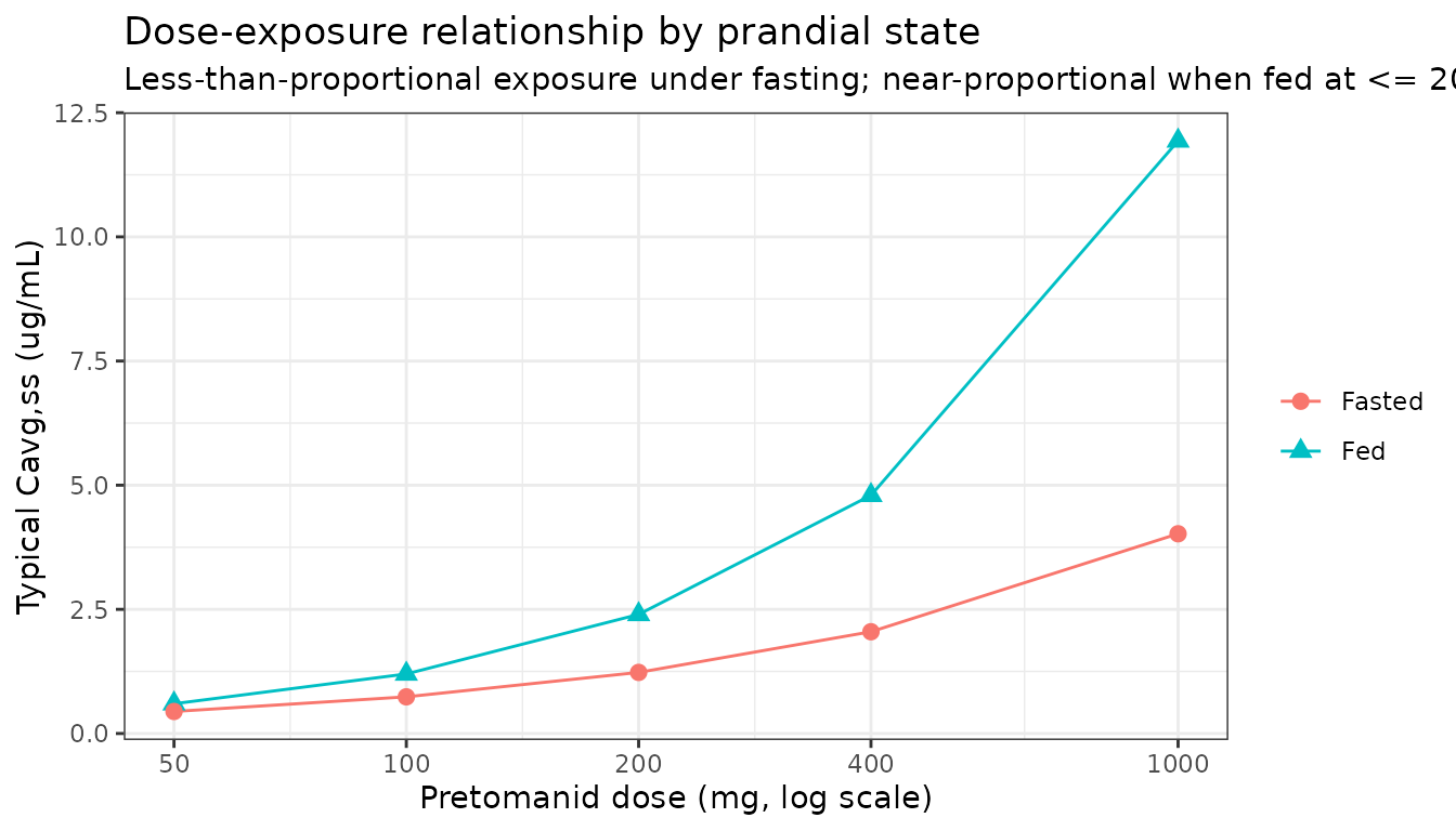
fed <- arms |> filter(fed == 1) |> arrange(dose)
fasted <- arms |> filter(fed == 0) |> arrange(dose)
# Salinger 2019 Abstract and Results: bioavailability in the fasted condition is
# "about half" that in the fed condition, and relative bioavailability decreases
# with increasing dose when fasted but NOT for doses <= 200 mg when fed.
ratio_200 <- fasted$f1[fasted$dose == 200] / fed$f1[fed$dose == 200]
cat("fasted:fed F1 ratio at 200 mg:", round(ratio_200, 3), "(Table 1: 0.513)\n")
#> fasted:fed F1 ratio at 200 mg: 0.513 (Table 1: 0.513)
stopifnot(abs(ratio_200 - 0.513) < 0.01)
# Fed F1 is flat at and below 200 mg (the dose term is gated on the fasted state
# and the 1000 mg fed indicator).
stopifnot(max(abs(fed$f1[fed$dose <= 200] - 1)) < 1e-8)
# Fasted F1 falls monotonically with dose; this is exact algebra, not a cohort.
stopifnot(all(diff(fasted$f1) < 0))
# Dose-normalised exposure therefore falls with dose when fasted.
dn <- fasted$cavg / fasted$dose
stopifnot(all(diff(dn) < 0), dn[length(dn)] / dn[1] < 0.75)
Assumptions, deviations and errata
Concentration units are ng/mL. Salinger 2019 tabulates exposures in ug/mL, but the residual-error magnitudes are calibrated to a dataset in ng/mL: an additive error variance of 11.5 is an SD of 3.39, which is implausible against a 2.4 ug/mL average concentration and sensible against 2,400 ng/mL. The model therefore computes
Cc <- 1000 * central / vc(mg/L to ng/mL) and declaresconcentration = "ng/mL". Every comparison in this vignette converts to ug/mL to match the paper’s tables.MTT ~ NC5is a boundary estimate, carried as published. Table 1 reports 6.95e-07 for this effect, which enters the model through a logarithm and so drives the mean transit time to about 1e-06 h in study NC-005 – an effectively instantaneous transit chain. Two independent checks confirm the reading rather than a transcription error. First, the reported confidence interval (-0.0350 to 0.0350) brackets zero, which is impossible for a positive parameter entering through a logarithm and is the signature of a parameter pinned at a boundary where the covariance step is meaningless. Second, Table S4 gives a medianMTT + 1/KAof 3.8 h for the NC-005 row while1/KAalone is 3.9 h, leaving no room for a transit delay. SettingSTUDY_NC005 = 1therefore produces a transit rate constant near 3e+06 1/h; this solves, but users should expect the chain to behave as a pass-through.The two later clearance arms are stored as sums. Table 1 reports the day-5 and Nix-TB week-6 clearance terms as additive increments (0.175 and 0.466 L/h) rather than as attained clearances, because the control stream writes them inside a single logarithm.
lcl_lateandlcl_late2name attained levels, so they hold 3.475 and 3.941 L/h; each in-file comment records the published increment and its confidence interval, which the summed level does not have.The clearance breakpoints are structural, not estimated.
ltclchange(96 h) andltclchange2(1008 h) arefixed()because the source defines them by a study-day / study-week conditional rather than fitting them.The day-5 step is keyed to time after the first dose, not to study membership. The source sets its steady-state indicator for study numbers 2, 5, 7, 10 and every patient study (> 100) from study day 5 onward – that enumeration is exactly the set of multiple-dose studies. The model uses
tafd() >= 96, which reproduces the source for any repeated-dose regimen. A single-dose simulation followed beyond 96 h will apply the step even though no multiple-dose study contributed such a record; single-dose simulations should be read over the first 96 h.The fasted F1 dose slope carries the random effect, per the control stream. Salinger 2019 Materials and Methods says “a random effect on the dose effect for fed subjects also significantly improved model fit”, but Table S3 multiplies
ETA(1)byFASTED, and both Table 1 and the ETA shrinkage footnote label the term “dose/fasted”. The control stream and the two tables agree, so the fasted reading is used and the Methods sentence is treated as a slip.FEDis the canonical covariate; the source column isFASTED. Every prandial effect is applied ase_..._..^(1 - FED), following theGoel_2016_Sonidegib.Rprecedent. The estimates are unchanged: they are fasted-versus-fed ratios either way.Interoccasion variability needs a study-specific occasion column. Occasions are defined per contributing study from trial length and sampling schedule (Table S1) – weeks 2 / 8 / 16 for Nix-TB, days 1-7 / 8-13 / 14-29 for the longer phase 1 studies, and so on.
OOC1/OOC2/OOC3must be assembled per Table S1; this vignette simulates occasion 1 only.The
Wline in the source$ERRORblock has a typo that does not affect the fit. Table S3 computes the weight for individual weighted residuals asW = SQRT(IPRED**(2*THETA(17))*SIGMA(1,1)**2 + SIGMA(2,2)**2), usingTHETA(17)(the moxifloxacin clearance effect) where the error power isTHETA(10), and squaring variances that are already variances.Wfeeds only theIWRESdiagnostic, neverY, so the published parameter estimates are unaffected. The model implements theYline, which correctly usesTHETA(10).Residual error is a power plus additive model. Table S3’s
Y = IPRED + EPS(1)*(IPRED + 1e-04)^THETA(10) + EPS(2)with a diagonal$SIGMAgives independent terms whose variances add, which is nlmixr2’scombined2(). The 1e-04 safeguard against0^poweris omitted as numerically negligible.No parameter value came from outside the paper. Every
ini()entry is from Salinger 2019 Table 1 or, for the two structural breakpoints, from the supplemental Table S3 control file. Nothing was digitised from a figure, obtained by correspondence, or carried from an upstream model. No erratum or corrigendum for this article was located.Covariates screened but not retained are recorded in the model file’s
covariatesDataExcludedmetadata rather thancovariateData: age, BMI, creatinine clearance, eGFR, ALT, AST, race, concomitant clofazimine, and the NC-002 and NC-006 study indicators. More than 99% of subjects had normal or only mildly impaired renal function, and less than 1% of parent drug was excreted in urine in two mass-balance studies.Published medians versus typical values. Table S4 reports medians over a simulated cohort; the primary gate in this vignette is deterministic. The random effects on clearance and volume are Box-Cox transformed and strongly right-skewed, so the two differ by a small reproducible offset. The three study-specific rows are gated separately because the Nix-TB Box-Cox shape of 26.0 makes that offset much larger – the paper’s own mean half-life for the TI/NR MDR row is 3.9e+96 h.