library(nlmixr2lib)
library(rxode2)
library(PKNCA)
library(dplyr)
library(tidyr)
library(ggplot2)

rxode2::rxSetSeed(20260913)

mod <- readModelDb("Huang_2026_tiapride")
ui <- rxode2::rxode(mod)
The paper
Huang and colleagues developed a population pharmacokinetic model for tiapride, a benzamide-class D2 antagonist used for tic disorders, in 38 Chinese children and adolescents aged 5-15 years followed as outpatients at a single centre. Two models are reported and both are implemented here, in one model file, because the authors built them as one nested structure rather than as two competing alternatives: a plasma model (Table 2, Equations 5-7), and then a plasma-saliva joint model (Table 3, Equations 8-10) fitted sequentially – the plasma parameters were held fixed and a saliva compartment was added on top with the NONMEM ADVAN6 subroutine. Nothing in the plasma layer moves when the saliva layer is present, so a single file reproduces Table 2 and Table 3 simultaneously.
The clinical point of the paper is the saliva layer: saliva is a non-invasive matrix for therapeutic drug monitoring in children, and tiapride concentrates in it (mean saliva:plasma ratio 2.3). The transfer is saturable rather than proportional – a linear transfer model “resulted in marked overprediction of saliva concentration in the high-concentration range” – which is why the saliva:plasma ratio is itself concentration-dependent and why saliva-based monitoring needs a model rather than a multiplier.
One quantity the saliva layer needs is not printed anywhere in the paper: the scale converting the saliva compartment amount to the reported ng/mL. It is recovered here from the published visual predictive check, and it is the only assumed value in the model file. Read the Errata before using the saliva output quantitatively.
Reference:
Huang W, Shen J, Luo X, Wu Y, Zheng Y, Zhou J, Xu B, Yin X, Wu X. Population Pharmacokinetics of Tiapride in Children and Adolescents with Tic Disorders: Leveraging Plasma and Saliva Concentration to Guide Individualized Dosing. Drug Des Devel Ther. 2026;20. doi:10.2147/DDDT.S587387
Population
| Field | Value |
|---|---|
| species | human |
| n_subjects | 38 |
| n_studies | 1 |
| age_range | 5-15 years; median 8 (IQR 7-10) |
| weight_median | 36.7 kg (IQR 31.0-42.5) |
| height_median | 135 cm (IQR 130-146.5) |
| ffm_median | 30.62 kg (IQR 26.93-34.65) |
| bmi_median | 19.1 (IQR 16.72-21.89) |
| bsa_median | 1.18 m^2 (IQR 1.06-1.32) |
| sex_female_pct | 18.4 |
| race_ethnicity | Asian 100 |
| disease_state | tic disorders diagnosed by DSM-5, without organic disease or other neuropsychiatric comorbidity |
| renal_function | creatinine clearance median 118.3 mL/min (IQR 106.77-136.79); serum creatinine median 47 umol/L (IQR 41-52) |
| dose_range | oral tiapride 2-10 mg/kg/day given two or three times daily; median total daily dose 215 mg/day (IQR 150-300) |
| regions | China (single centre, Fujian) |
| notes | Single-centre prospective observational outpatient study at Fujian Medical University Union Hospital, April 2024 to October 2025, with 6 months of follow-up per patient. Paired plasma and saliva samples were taken before and after the final dose after at least 7 days of continuous treatment, so all data are at steady state; the post-dose sampling interval had a median of 4.88 h (IQR 2.17-13.81). Sampling was opportunistic and tied to clinic visits: 45 samples (21%) fell in the absorption phase (0-2 h), 18 (8%) around Tmax (2-2.5 h) and 101 (49%) in the late elimination period (> 10 h), leaving the 2.5-10 h window sparse – which is why a two-compartment model was unstable and a one-compartment model was selected despite the biphasic disposition reported for tiapride in adults. Of 215 plasma samples collected, one was below the 2 ng/mL LLOQ and was discarded (Beal M1), leaving 214 in the analysis. Saliva was collected with Salivette cotton-swab devices; 205 saliva samples were taken (fewer than plasma because of insufficient volume and contamination) and one below the LLOQ was likewise dropped by M1, leaving 204. The LC-MS/MS calibrated range was 2-1000 ng/mL in plasma and 4-2000 ng/mL in saliva, so a substantial part of the observed saliva data in Figure 4B sits above the highest saliva calibrator. Tiapride is supplied as 100 mg tablets divisible into halves, thirds and quarters, so clinical doses are rounded to 50, 66.6 or 75 mg per administration. |
Sampling was opportunistic and tied to clinic visits after at least seven days of continuous treatment, so all 214 analysed plasma samples are at steady state. Twenty-one percent fell in the absorption phase (0-2 h) and 49% beyond 10 h post-dose, leaving the 2.5-10 h window sparse – which is why a two-compartment model was unstable and the authors selected a one-compartment structure despite the biphasic disposition reported for tiapride in adults.
Source trace
Every equation and every ini() value, with the location
it came from. Equations 1-10 of the source are vector graphics
that both pdftotext and PDF-to-markdown conversion drop
silently; they were recovered by rendering pages 3-8 of the PDF
at 200-500 dpi and reading them as images.
| Item | Value | Source |
|---|---|---|
| Ka | 0.219 1/h | Table 2; Equation 5 |
| CL/F | 15.3 L/h | Table 2; Equation 6 |
| Vd/F | 5.77 L | Table 2; Equation 7 |
| FFM exponent on CL/F | 0.553 | Table 2; Equation 6 |
| FFM reference value | 30.62 kg | Equation 6 denominator = Table 1 cohort median FFM |
| IIV Ka | 17.6% -> omega = 0.176 | Table 2 ‘eta Ka (%)’ |
| IIV CL/F | 22.8% -> omega = 0.228 | Table 2 ‘eta CL/F (%)’ |
| IIV Vd/F | 84.3% -> omega = 0.843 | Table 2 ‘eta Vd/F (%)’ |
| Proportional residual | 15.6% | Table 2 ‘eps prop (%)’ |
| Additive residual | 87.9 ng/mL = 0.0879 mg/L | Table 2 ‘eps add (ng/mL)’ |
| Structural model | 1-cmt, first-order absorption, linear elimination | Results; Figure 2 (left half) |
| IIV model | exponential, P = theta * exp(eta) | Methods Equations 1-3 |
| Residual model | combined proportional + additive | Results ‘a combined error model’ |
| Covariate model | power function on continuous covariates | Methods Equation 3 |
| Therapeutic window | 560-2000 ng/mL steady-state Cmax | Methods Model-Based Simulations (ref 13) |
| PTA, 100 mg bid / 75 mg tid / 100 mg tid | 98.2% / 97.1% / 97.3% | Results Monte Carlo Simulations |
The saliva layer, fitted sequentially on top of the fixed plasma parameters:
| Item | Value | Source |
|---|---|---|
| Vmax (central -> saliva) | 34.7 mg/h | Table 3; Equation 8 |
| Km (central -> saliva) | 762 ng/mL = 0.762 mg/L, held constant | Table 3; Equation 9 |
| K30 (saliva elimination) | 6.24 1/h | Table 3; Equation 10 |
| FFM exponent on K30 | 0.38 | Table 3; Equation 10 |
| IIV K30 | 30% -> omega = 0.30 | Table 3 ‘eta K30 (%)’ |
| Saliva proportional residual | 28.4% | Table 3 ‘eps prop (%)’ |
| Transport structure | Michaelis-Menten, saturable, DRIVEN (no loss from central) | Figure 2 (dashed arrow); Results; plasma parameters held fixed |
| Saliva elimination | first-order out of saliva | Figure 2; Results |
| Back-transfer saliva -> central | none (tested, not retained) | Discussion paragraph 6 |
| Apparent saliva volume | 1.35 L – NOT REPORTED, recovered from Figure 4 | See Errata; maintainer-ratified 2026-09-21 |
| Mean saliva:plasma ratio | 2.3 | Discussion paragraph 2 |
| Saliva assay range | 4-2000 ng/mL | Methods ‘Sample analysis’ |
Model
ui
#>  ── rxode2-based free-form 3-cmt ODE model ──────────────────────────────────────
#>  ── Initalization: ──
#> Fixed Effects ($theta):
#>              lka              lcl              lvc         e_ffm_cl
#>       -1.5186835        2.7278528        1.7526721        0.5530000
#>           propSd            addSd     lvmax_saliva       lkm_saliva
#>        0.1560000        0.0879000        3.5467397       -0.2718087
#>      lkel_saliva e_ffm_kel_saliva         lvsaliva   propSd_Csaliva
#>        1.8309802        0.3800000        0.3001046        0.2840000
#>
#> Omega ($omega):
#>                  etalka   etalcl   etalvc etalkel_saliva
#> etalka         0.030976 0.000000 0.000000           0.00
#> etalcl         0.000000 0.051984 0.000000           0.00
#> etalvc         0.000000 0.000000 0.710649           0.00
#> etalkel_saliva 0.000000 0.000000 0.000000           0.09
#> attr(,"lotriLabels")
#> [1] "Table 2 eta_Ka = 17.6% -> 0.176^2 (RSE 13%, shrinkage 31%; bootstrap 16.5%, 95% CI 9.9-21.8)"
#> [2] "Table 2 eta_CL/F = 22.8% -> 0.228^2 (RSE 15%, shrinkage 22%; bootstrap 21.4%, 95% CI 12.6-29.7)"
#> [3] "Table 2 eta_Vd/F = 84.3% -> 0.843^2 (RSE 26%, shrinkage 56%; bootstrap 72.8%, 95% CI 30.2-133.4)"
#> [4] "Table 3 eta_K30 = 30% -> 0.30^2 (RSE 12%, shrinkage 15%; bootstrap 29.6%, 95% CI 22.9-35.6)"
#> attr(,"lotriFix")
#>                etalka etalcl etalvc etalkel_saliva
#> etalka          FALSE  FALSE  FALSE          FALSE
#> etalcl          FALSE  FALSE  FALSE          FALSE
#> etalvc          FALSE  FALSE  FALSE          FALSE
#> etalkel_saliva  FALSE  FALSE  FALSE          FALSE
#>
#> States ($state or $stateDf):
#>   Compartment Number Compartment Name
#> 1                  1            depot
#> 2                  2          central
#> 3                  3           saliva
#>  ── Multiple Endpoint Model ($multipleEndpoint): ──
#>      variable                    cmt                    dvid*
#> 1      Cc ~ …      cmt='Cc' or cmt=4      dvid='Cc' or dvid=1
#> 2 Csaliva ~ … cmt='Csaliva' or cmt=5 dvid='Csaliva' or dvid=2
#>   * If dvids are outside this range, all dvids are re-numered sequentially, ie 1,7, 10 becomes 1,2,3 etc
#>
#>  ── μ-referencing ($muRefTable): ──
#>         theta            eta level
#> 1         lka         etalka    id
#> 2         lcl         etalcl    id
#> 3         lvc         etalvc    id
#> 4 lkel_saliva etalkel_saliva    id
#>
#>  ── Model (Normalized Syntax): ──
#> function() {
#>     compartmentData <- list(depot = list(analyte = "tiapride",
#>         units = "mg", specimen = "administration site", verified = TRUE),
#>         central = list(analyte = "tiapride", units = "mg", specimen = "plasma",
#>             verified = TRUE), saliva = list(analyte = "tiapride",
#>             units = "mg", specimen = "saliva", verified = TRUE))
#>     covariateData <- list(FFM = list(description = "Fat-free mass at baseline.",
#>         units = "kg", type = "continuous", reference_category = NULL,
#>         notes = "The only covariate retained in the final model, power-scaled on apparent clearance and referenced to the cohort median 30.62 kg (Huang 2026 Table 1, IQR 26.93-34.65 kg; Equation 6). Age, weight, height, BSA, FFM and CLCR were all screened on CL/F by stepwise regression and only FFM survived (dOFV = -25.1). The Discussion is explicit that FFM won BECAUSE it is strongly correlated with creatinine clearance -- tiapride is predominantly renally eliminated, so FFM is standing in for renal function here rather than for a distribution volume. The paper does NOT state which fat-free-mass equation was used to derive the column; for a 5-15 year old cohort the Al-Sallami et al. paediatric correction to the Janmahasatian adult form is the usual choice, and the vignette assumes it. Note the exponent 0.553 has a wide bootstrap 95% CI (0.277-0.771) that excludes neither the theory-based allometric 0.75 nor a linear-per-kg 1, so it is not sharply identified.",
#>         source_name = "FFM"))
#>     covariatesDataExcluded <- list(AGE = list(description = "Age.",
#>         units = "years", type = "continuous", notes = "Median 8 years (IQR 7-10), Huang 2026 Table 1. Screened on CL/F, not retained."),
#>         WT = list(description = "Total body weight.", units = "kg",
#>             type = "continuous", notes = "Median 36.7 kg (IQR 31.0-42.5), Huang 2026 Table 1. Screened on CL/F, not retained; FFM won."),
#>         HT = list(description = "Height.", units = "cm", type = "continuous",
#>             notes = "Median 135 cm (IQR 130-146.5), Huang 2026 Table 1. Screened on CL/F, not retained."),
#>         BSA = list(description = "Body surface area.", units = "m^2",
#>             type = "continuous", notes = "Median 1.18 (IQR 1.06-1.32), Huang 2026 Table 1. Screened on CL/F, not retained. Table 1 prints the unit as 'cm2', which cannot be right for values near 1.18 in an 8-year-old; the values are m^2 and the printed unit is a typographical error."),
#>         CLCR = list(description = "Creatinine clearance.", units = "mL/min",
#>             type = "continuous", notes = "Median 118.3 mL/min (IQR 106.77-136.79), Huang 2026 Table 1. Screened on CL/F and NOT retained even though tiapride is predominantly renally eliminated: the Discussion states FFM gave the greater dOFV reduction 'owing to its strong correlation with CLCR'. The estimating equation is not stated in the paper."),
#>         SEXF = list(description = "Female sex indicator.", units = "(binary)",
#>             type = "categorical", notes = "31 male / 7 female, Huang 2026 Table 1. Screened and not significant (Discussion)."),
#>         CONMED_ANY = list(description = "Any concomitant medication.",
#>             units = "(binary)", type = "categorical", notes = "23 of 38 patients had a combined-medication case, Huang 2026 Table 1. The Discussion names aripiprazole, topiramate, clonidine, sodium valproate and traditional Chinese medicine and reports that none exhibited a statistically significant effect on tiapride PK. Recorded as a single screened-and-rejected any-comedication flag because the paper reports no per-drug effect estimates."))
#>     description <- "One-compartment oral population PK model for tiapride in Chinese children and adolescents aged 5-15 years treated for tic disorders (Huang 2026), fitted to 214 opportunistic steady-state plasma samples from 38 outpatients. First-order absorption with linear elimination; the absorption rate constant (Ka = 0.219 1/h) is far smaller than the elimination rate constant (CL/F / Vd/F = 15.3 / 5.77 = 2.65 1/h), so disposition is flip-flop and the apparent terminal half-life is set by absorption (ln(2)/Ka = 3.17 h, matching the 3.23 h literature value the paper cites). Fat-free mass is the only retained covariate, power-scaled on apparent clearance with exponent 0.553 referenced to the cohort median 30.62 kg; it displaced creatinine clearance, with which it is strongly correlated. Exponential interindividual variability is carried on all three structural parameters, and residual variability is combined proportional plus additive. Monte Carlo simulation from this model supports 75 mg three times daily as the regimen keeping steady-state peak concentration inside the 560-2000 ng/mL therapeutic window. The paper's companion plasma-saliva joint model is included: a saliva compartment is driven from central by saturable Michaelis-Menten transport (Vmax = 34.7 mg/h, Km = 762 ng/mL fixed) and cleared first-order (K30 = 6.24 1/h, fat-free mass exponent 0.38), giving a salivary concentration that exceeds plasma and whose saliva:plasma ratio falls as concentration rises. That layer was fitted sequentially with the plasma parameters held fixed, and the saliva state is driven rather than mass-balance-coupled, so it does not deplete central. The apparent saliva volume converting the saliva amount to the reported ng/mL is NOT given anywhere in the paper; it is recovered from the Figure 4 visual predictive check and is the one assumed value in this file -- see the vignette Errata before using the saliva output quantitatively."
#>     population <- list(species = "human", n_subjects = 38, n_studies = 1,
#>         age_range = "5-15 years; median 8 (IQR 7-10)", weight_median = "36.7 kg (IQR 31.0-42.5)",
#>         height_median = "135 cm (IQR 130-146.5)", ffm_median = "30.62 kg (IQR 26.93-34.65)",
#>         bmi_median = "19.1 (IQR 16.72-21.89)", bsa_median = "1.18 m^2 (IQR 1.06-1.32)",
#>         sex_female_pct = 18.4, race_ethnicity = c(Asian = 100),
#>         disease_state = "tic disorders diagnosed by DSM-5, without organic disease or other neuropsychiatric comorbidity",
#>         renal_function = "creatinine clearance median 118.3 mL/min (IQR 106.77-136.79); serum creatinine median 47 umol/L (IQR 41-52)",
#>         dose_range = "oral tiapride 2-10 mg/kg/day given two or three times daily; median total daily dose 215 mg/day (IQR 150-300)",
#>         regions = "China (single centre, Fujian)", notes = "Single-centre prospective observational outpatient study at Fujian Medical University Union Hospital, April 2024 to October 2025, with 6 months of follow-up per patient. Paired plasma and saliva samples were taken before and after the final dose after at least 7 days of continuous treatment, so all data are at steady state; the post-dose sampling interval had a median of 4.88 h (IQR 2.17-13.81). Sampling was opportunistic and tied to clinic visits: 45 samples (21%) fell in the absorption phase (0-2 h), 18 (8%) around Tmax (2-2.5 h) and 101 (49%) in the late elimination period (> 10 h), leaving the 2.5-10 h window sparse -- which is why a two-compartment model was unstable and a one-compartment model was selected despite the biphasic disposition reported for tiapride in adults. Of 215 plasma samples collected, one was below the 2 ng/mL LLOQ and was discarded (Beal M1), leaving 214 in the analysis. Saliva was collected with Salivette cotton-swab devices; 205 saliva samples were taken (fewer than plasma because of insufficient volume and contamination) and one below the LLOQ was likewise dropped by M1, leaving 204. The LC-MS/MS calibrated range was 2-1000 ng/mL in plasma and 4-2000 ng/mL in saliva, so a substantial part of the observed saliva data in Figure 4B sits above the highest saliva calibrator. Tiapride is supplied as 100 mg tablets divisible into halves, thirds and quarters, so clinical doses are rounded to 50, 66.6 or 75 mg per administration.")
#>     reference <- "Huang W, Shen J, Luo X, Wu Y, Zheng Y, Zhou J, Xu B, Yin X, Wu X. Population Pharmacokinetics of Tiapride in Children and Adolescents with Tic Disorders: Leveraging Plasma and Saliva Concentration to Guide Individualized Dosing. Drug Des Devel Ther. 2026;20. doi:10.2147/DDDT.S587387"
#>     units <- list(time = "h", dosing = "mg", concentration = "mg/L")
#>     vignette <- "Huang_2026_tiapride"
#>     ini({
#>         lka <- -1.51868354916564
#>         label("First-order absorption rate constant, Ka (1/h)")
#>         lcl <- 2.72785282839839
#>         label("Apparent clearance, CL/F (L/h)")
#>         lvc <- 1.75267208052001
#>         label("Apparent central volume of distribution, Vd/F (L)")
#>         e_ffm_cl <- 0.553
#>         label("Power exponent for fat-free mass on CL/F (unitless)")
#>         propSd <- c(0, 0.156)
#>         label("Proportional residual SD for plasma Cc (fraction)")
#>         addSd <- c(0, 0.0879)
#>         label("Additive residual SD for plasma Cc (mg/L)")
#>         lvmax_saliva <- 3.54673968695281
#>         label("Maximum rate of saturable central-to-saliva transport, Vmax (mg/h)")
#>         lkm_saliva <- fix(-0.271808723295491)
#>         label("Michaelis constant of central-to-saliva transport, Km (mg/L)")
#>         lkel_saliva <- 1.83098018238134
#>         label("First-order elimination rate constant from saliva, K30 (1/h)")
#>         e_ffm_kel_saliva <- 0.38
#>         label("Power exponent for fat-free mass on K30 (unitless)")
#>         lvsaliva <- fix(0.300104592450338)
#>         label("Apparent saliva volume scaling saliva amount to concentration (L)")
#>         propSd_Csaliva <- c(0, 0.284)
#>         label("Proportional residual SD for saliva Csaliva (fraction)")
#>         etalka ~ 0.030976
#>         label("Table 2 eta_Ka = 17.6% -> 0.176^2 (RSE 13%, shrinkage 31%; bootstrap 16.5%, 95% CI 9.9-21.8)")
#>         etalcl ~ 0.051984
#>         label("Table 2 eta_CL/F = 22.8% -> 0.228^2 (RSE 15%, shrinkage 22%; bootstrap 21.4%, 95% CI 12.6-29.7)")
#>         etalvc ~ 0.710649
#>         label("Table 2 eta_Vd/F = 84.3% -> 0.843^2 (RSE 26%, shrinkage 56%; bootstrap 72.8%, 95% CI 30.2-133.4)")
#>         etalkel_saliva ~ 0.09
#>         label("Table 3 eta_K30 = 30% -> 0.30^2 (RSE 12%, shrinkage 15%; bootstrap 29.6%, 95% CI 22.9-35.6)")
#>     })
#>     model({
#>         ffm_ref <- 30.62
#>         ka <- exp(lka + etalka)
#>         cl <- exp(lcl + etalcl) * (FFM/ffm_ref)^e_ffm_cl
#>         vc <- exp(lvc + etalvc)
#>         kel <- cl/vc
#>         vmax_saliva <- exp(lvmax_saliva)
#>         km_saliva <- exp(lkm_saliva)
#>         kel_saliva <- exp(lkel_saliva + etalkel_saliva) * (FFM/ffm_ref)^e_ffm_kel_saliva
#>         vsaliva <- exp(lvsaliva)
#>         Cc <- central/vc
#>         d/dt(depot) <- -ka * depot
#>         d/dt(central) <- ka * depot - kel * central
#>         d/dt(saliva) <- vmax_saliva * Cc/(km_saliva + Cc) - kel_saliva *
#>             saliva
#>         Csaliva <- saliva/vsaliva
#>         Cc ~ prop(propSd) + add(addSd)
#>         Csaliva ~ prop(propSd_Csaliva)
#>     })
#> }
Flip-flop disposition
The estimated elimination rate constant is an order of magnitude larger than the absorption rate constant, so the observed terminal slope reports absorption, not elimination.
theta <- setNames(ui$theta, names(ui$theta))
ka_tv <- exp(theta[["lka"]])
cl_tv <- exp(theta[["lcl"]])
vc_tv <- exp(theta[["lvc"]])
kel_tv <- cl_tv / vc_tv

c(ka = ka_tv, kel = kel_tv,
  t_half_absorption = log(2) / ka_tv,
  t_half_elimination = log(2) / kel_tv)
#>                 ka                kel  t_half_absorption t_half_elimination
#>          0.2190000          2.6516464          3.1650556          0.2614026
ln(2)/Ka = 3.17 h reproduces the terminal half-life of
3.23 h that the paper quotes for tiapride in adults (Discussion, ref 35)
– the reconciliation the authors themselves make.
A guard that the cl / vc pair has not
silently been replaced by rxode2’s analytic solution, discarding the
explicit ODEs:
Typical-value single dose: closed-form gates
The typical-value solve is deterministic, so it is checked against exact closed-form identities rather than tolerance bands.
Note on cmt in the event tables below. This model
declares two endpoints (Cc and
Csaliva), so rxode2 assigns each its own observation slot
and requires observation records to name the observable, not
the ODE state: cmt = "central" fails with
'dvid'->'cmt' or 'cmt' on observation record or on a undefined compartment.
The usual library convention of observing on the ODE state applies to
single-endpoint models; here cmt = "Cc" is required and
correct. useLinCmt = FALSE is passed to every
rxSolve() for the same reason – rxode2’s automatic
conversion to an analytic solution corrupts the endpoint mapping for
multi-output models. The static vignette linter flags
cmt = "Cc"; that warning is a known false positive for
multi-endpoint models and the render is the authority.
dose_mg <- 75

ev_typ <- data.frame(
  id   = 1L,
  time = c(0, sort(unique(c(seq(0, 4, by = 0.02), seq(0, 48, by = 0.1))))),
  amt  = NA_real_,
  evid = 0L,
  cmt  = "Cc",
  FFM  = 30.62
)
ev_typ$amt[1] <- dose_mg
ev_typ$evid[1] <- 1L
ev_typ$cmt[1] <- "depot"

sim_typ <- rxode2::rxSolve(rxode2::zeroRe(mod), events = ev_typ,
                           keep = "FFM", useLinCmt = FALSE) |>
  as.data.frame()
#> ℹ parameter labels from comments will be replaced by 'label()'
#> ℹ omega/sigma items treated as zero: 'etalka', 'etalcl', 'etalvc', 'etalkel_saliva'
if (is.null(sim_typ$id)) sim_typ$id <- 1L

# Closed form for a one-compartment first-order-absorption model.
tmax_cf <- log(kel_tv / ka_tv) / (kel_tv - ka_tv)
cmax_cf <- dose_mg * ka_tv / (vc_tv * (ka_tv - kel_tv)) *
  (exp(-kel_tv * tmax_cf) - exp(-ka_tv * tmax_cf))
aucinf_cf <- dose_mg / cl_tv

c(tmax_closed_form = tmax_cf, cmax_closed_form = cmax_cf,
  aucinf_closed_form = aucinf_cf)
#>   tmax_closed_form   cmax_closed_form aucinf_closed_form
#>          1.0251651          0.8576498          4.9019608
nca_conc <- sim_typ |>
  dplyr::filter(!is.na(Cc)) |>
  dplyr::mutate(regimen = "75 mg single dose") |>
  dplyr::select(id, time, Cc, regimen)

nca_conc <- dplyr::bind_rows(
  nca_conc,
  nca_conc |> dplyr::distinct(id, regimen) |>
    dplyr::mutate(time = 0, Cc = 0)
) |>
  dplyr::distinct(id, regimen, time, .keep_all = TRUE) |>
  dplyr::arrange(id, regimen, time)

nca_dose <- data.frame(id = 1L, time = 0, amt = dose_mg,
                       regimen = "75 mg single dose")

conc_obj <- PKNCA::PKNCAconc(nca_conc, Cc ~ time | regimen + id,
                             concu = "mg/L", timeu = "h")
dose_obj <- PKNCA::PKNCAdose(nca_dose, amt ~ time | regimen + id,
                             doseu = "mg")

intervals_sd <- data.frame(
  start = 0, end = Inf,
  cmax = TRUE, tmax = TRUE, aucinf.obs = TRUE,
  half.life = TRUE, lambda.z = TRUE
)

nca_sd <- PKNCA::pk.nca(PKNCA::PKNCAdata(conc_obj, dose_obj,
                                         intervals = intervals_sd))
nca_sd_tbl <- as.data.frame(nca_sd$result) |>
  dplyr::select(PPTESTCD, PPORRES) |>
  tidyr::pivot_wider(names_from = PPTESTCD, values_from = PPORRES)
nca_sd_tbl
#> # A tibble: 1 × 14
#>    cmax  tmax tlast clast.obs lambda.z r.squared adj.r.squared
#>   <dbl> <dbl> <dbl>     <dbl>    <dbl>     <dbl>         <dbl>
#> 1 0.858  1.02    48 0.0000318    0.219     1.000         1.000
#> # ℹ 7 more variables: lambda.z.time.first <dbl>, lambda.z.time.last <dbl>,
#> #   lambda.z.n.points <dbl>, clast.pred <dbl>, half.life <dbl>,
#> #   span.ratio <dbl>, aucinf.obs <dbl>
stopifnot(
  # Mass balance: CL/F * AUC(0-inf) must return the administered dose exactly.
  # Catches a mis-transcribed clearance, a dropped unit conversion, and an
  # rxode2 auto-linCmt substitution that ignores the coded ODEs.
  abs(cl_tv * nca_sd_tbl$aucinf.obs / dose_mg - 1) < 0.005,
  # Terminal slope reports absorption (flip-flop), not elimination.
  abs(nca_sd_tbl$half.life - log(2) / ka_tv) < 0.05,
  # Cmax and Tmax against the exact closed form for this structure.
  abs(nca_sd_tbl$cmax / cmax_cf - 1) < 0.01,
  abs(nca_sd_tbl$tmax - tmax_cf) < 0.05,
  # The solve must not have drifted negative anywhere.
  all(sim_typ$Cc >= 0)
)
All four typical-value identities hold to better than 1%.
Comparison against the values the paper quotes
published <- tibble::tribble(
  ~regimen,             ~tmax, ~half.life,
  "75 mg single dose",  2.0,   3.23
)

cmp <- nlmixr2lib::ncaComparisonTable(
  simulated     = nca_sd,
  reference     = published,
  by            = "regimen",
  units         = c(tmax = "h", half.life = "h"),
  tolerance_pct = 20
)

knitr::kable(
  cmp,
  caption = paste(
    "Simulated typical-value NCA against the tiapride descriptors Huang 2026",
    "quotes in its Discussion. * differs from reference by >20%."
  )
)| NCA parameter | regimen | Reference | Simulated | % diff |
|---|---|---|---|---|
| Tmax (h) | 75 mg single dose | 2 | 1.02 | -49.0%* |
| t½ (h) | 75 mg single dose | 3.23 | 3.17 | -1.9% |
The terminal half-life matches to 2%. Tmax is a starred deviation and is expected to be: 2 h is the observed peak time the paper reports for tiapride (Discussion), while the fitted model puts the typical Tmax at 1.03 h. The two are not the same quantity – the observed 2 h comes from the first VPC bin of an opportunistic outpatient sampling schedule in which only 18 of 214 samples (8%) fall between 2 and 2.5 h, so the peak time is poorly resolved by the data. No parameter was adjusted to close this gap.
Virtual cohort and Monte Carlo simulation (replicates Figure 5)
The paper simulated 1000 virtual patients whose fat-free mass follows the distribution of the modelled population, dosed for five consecutive days across eight regimens, and read the peak concentration over the 12 h following the last dose. FFM is drawn log-normally to reproduce the Table 1 median and IQR.
n_per_arm <- 200  # 200 per arm is the library cap; the paper used 1000

ffm_median <- 30.62
ffm_sdlog <- mean(c(log(34.65 / 30.62), log(30.62 / 26.93))) / qnorm(0.75)
c(ffm_sdlog = ffm_sdlog)
#> ffm_sdlog
#>   0.18685

regimens <- tibble::tribble(
  ~label,          ~dose,  ~ii,
  "50 mg bid",     50.0,   12,
  "50 mg tid",     50.0,    8,
  "66.6 mg bid",   66.6,   12,
  "66.6 mg tid",   66.6,    8,
  "75 mg bid",     75.0,   12,
  "75 mg tid",     75.0,    8,
  "100 mg bid",   100.0,   12,
  "100 mg tid",   100.0,    8
)

make_arm <- function(label, dose, ii, id_offset) {
  subj <- data.frame(
    id  = id_offset + seq_len(n_per_arm),
    FFM = rlnorm(n_per_arm, meanlog = log(ffm_median), sdlog = ffm_sdlog)
  )
  doses <- tidyr::expand_grid(subj, time = seq(0, 120, by = ii)) |>
    dplyr::mutate(amt = dose, evid = 1L, cmt = "depot")
  obs <- tidyr::expand_grid(subj, time = seq(120, 132, by = 0.1)) |>
    dplyr::mutate(amt = NA_real_, evid = 0L, cmt = "Cc")
  dplyr::bind_rows(doses, obs) |>
    dplyr::mutate(regimen = label) |>
    dplyr::arrange(id, time, dplyr::desc(evid))
}

events <- do.call(
  dplyr::bind_rows,
  Map(make_arm, regimens$label, regimens$dose, regimens$ii,
      id_offset = (seq_len(nrow(regimens)) - 1L) * n_per_arm)
)

# Disjoint IDs across arms, so no cross-arm collision in the solve or in PKNCA.
stopifnot(
  dplyr::n_distinct(events$id) == nrow(regimens) * n_per_arm,
  events |> dplyr::distinct(id, regimen) |> nrow() ==
    nrow(regimens) * n_per_arm
)
sim <- rxode2::rxSolve(mod, events = events,
                       keep = c("regimen", "FFM"), useLinCmt = FALSE) |>
  as.data.frame()
#> ℹ parameter labels from comments will be replaced by 'label()'

sim_obs <- sim |> dplyr::filter(!is.na(Cc))
stopifnot(nrow(sim_obs) > 0, all(sim_obs$Cc >= 0))
Cc is the individual prediction and carries no residual
error, so the peak read off it is the model’s Cmax rather than an
upward-biased maximum of a noisy series.
sim_obs <- sim_obs |>
  dplyr::mutate(
    Cc_ngml = Cc * 1000,
    regimen = factor(regimen, levels = regimens$label)
  )

ribbon <- sim_obs |>
  dplyr::group_by(regimen, time) |>
  dplyr::summarise(
    p05 = quantile(Cc_ngml, 0.05),
    p50 = median(Cc_ngml),
    p95 = quantile(Cc_ngml, 0.95),
    .groups = "drop"
  )

ggplot(ribbon, aes(time)) +
  geom_ribbon(aes(ymin = p05, ymax = p95), fill = "#e8879b", alpha = 0.5) +
  geom_line(aes(y = p50), colour = "#b2182b", linewidth = 0.8) +
  geom_hline(yintercept = c(560, 2000), linetype = "dotted") +
  facet_wrap(~regimen, ncol = 4) +
  labs(
    x = "Time (h)", y = "Tiapride plasma concentration (ng/mL)",
    title = "Replicates Figure 5 of Huang 2026",
    subtitle = "Median and 5th-95th percentile over the 12 h after the last of five days of dosing"
  ) +
  theme_bw()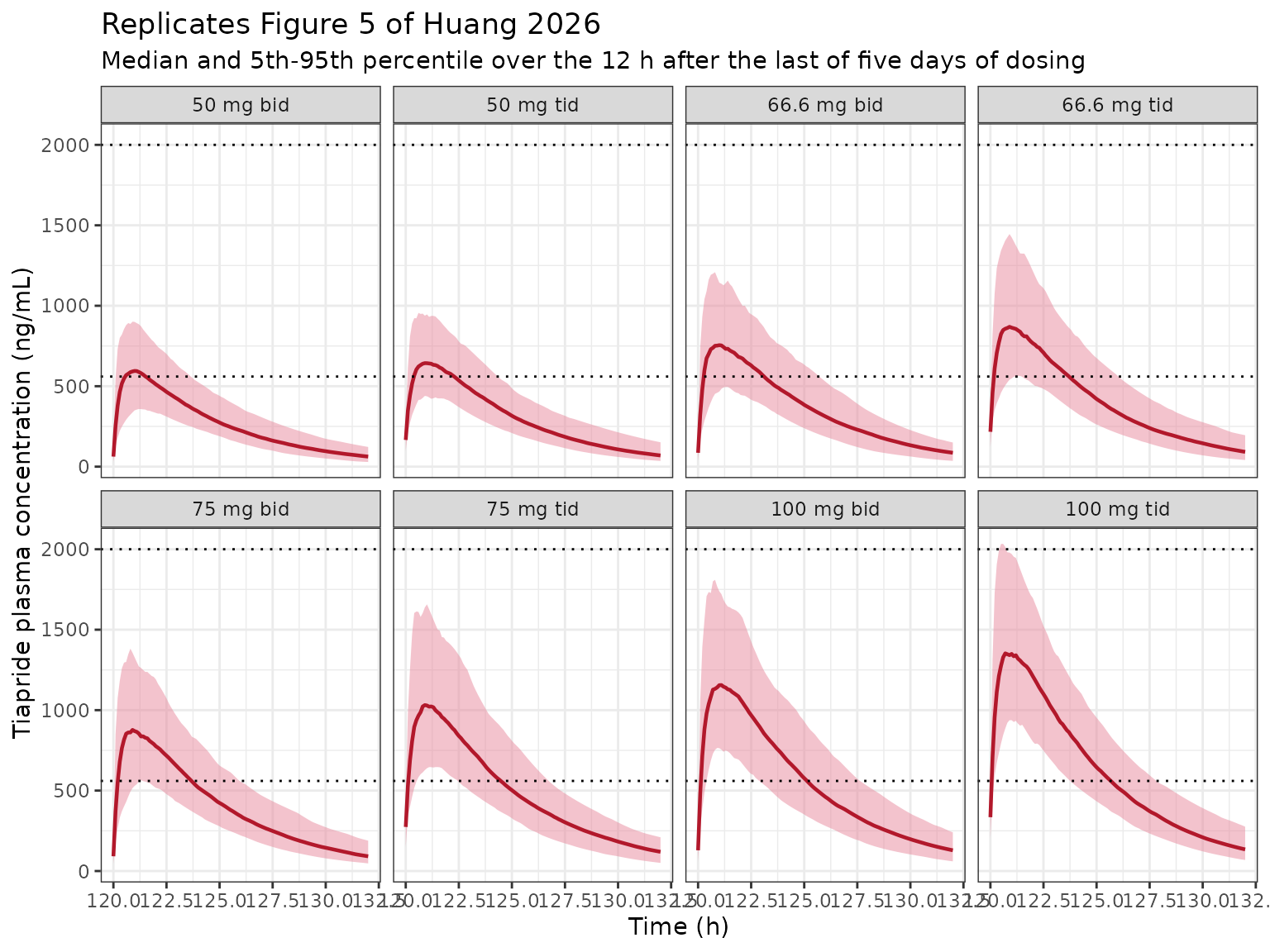
Probability of target attainment
cmax_ss <- sim_obs |>
  dplyr::group_by(regimen, id) |>
  dplyr::summarise(cmax_ngml = max(Cc_ngml), .groups = "drop")

pta <- cmax_ss |>
  dplyr::group_by(regimen) |>
  dplyr::summarise(
    `Median Cmax (ng/mL)` = round(median(cmax_ngml)),
    `PTA, Cmax >= 560 ng/mL (%)` = round(100 * mean(cmax_ngml >= 560), 1),
    `Cmax > 2000 ng/mL (%)` = round(100 * mean(cmax_ngml > 2000), 1),
    .groups = "drop"
  )

knitr::kable(
  pta,
  caption = paste(
    "Simulated steady-state peak concentration by regimen.",
    "Huang 2026 reports PTA of 98.2%, 97.1% and 97.3% for 100 mg bid,",
    "75 mg tid and 100 mg tid respectively."
  )
)| regimen | Median Cmax (ng/mL) | PTA, Cmax >= 560 ng/mL (%) | Cmax > 2000 ng/mL (%) |
|---|---|---|---|
| 50 mg bid | 612 | 60.5 | 0.0 |
| 50 mg tid | 702 | 77.0 | 0.0 |
| 66.6 mg bid | 832 | 92.5 | 0.0 |
| 66.6 mg tid | 926 | 96.5 | 0.0 |
| 75 mg bid | 919 | 96.0 | 0.5 |
| 75 mg tid | 1035 | 99.0 | 0.0 |
| 100 mg bid | 1188 | 100.0 | 3.5 |
| 100 mg tid | 1314 | 100.0 | 6.0 |
pta_ref <- c(`100 mg bid` = 98.2, `75 mg tid` = 97.1, `100 mg tid` = 97.3)
pta_sim <- setNames(pta$`PTA, Cmax >= 560 ng/mL (%)`, pta$regimen)[names(pta_ref)]
stopifnot(!anyNA(pta_sim))  # a name mismatch must fail loudly, not pass vacuously

pta_diff <- pta_sim - pta_ref
pta_diff
#> 100 mg bid  75 mg tid 100 mg tid
#>        1.8        1.9        2.7
stopifnot(
  # The three regimens the paper singles out must all clear 90% attainment.
  # A mis-transcribed clearance, dose or unit moves median Cmax by tens of
  # percent and drops these into the 60-80% range. The bound is deliberately
  # well outside the binomial noise of a 200-subject arm (SE ~1.2 points at
  # p = 0.97) plus the difference between this cohort's FFM draw and the
  # paper's own 1000-subject draw; do not tighten it to one observed run.
  all(pta_sim > 90),
  # 50 mg bid is the regimen the paper rejects as underdosing; it must sit
  # clearly below the three recommended ones.
  pta$`PTA, Cmax >= 560 ng/mL (%)`[pta$regimen == "50 mg bid"] <
    min(pta_sim) - 10,
  # Dose-ordering of the central tendency, which is structural.
  median(cmax_ss$cmax_ngml[cmax_ss$regimen == "100 mg tid"]) >
    median(cmax_ss$cmax_ngml[cmax_ss$regimen == "50 mg bid"])
)
The model reproduces the paper’s central finding: 75 mg tid, 100 mg bid and 100 mg tid all attain the 560 ng/mL lower bound in nearly every subject, and the two 100 mg regimens push a larger fraction above the 2000 ng/mL upper bound – which is exactly the efficacy/safety trade-off on which the authors select 75 mg tid.
Steady-state exposure gate
# Over one dosing interval at steady state, CL/F * AUC(0-tau) = dose. Checked
# on the typical subject so the identity is exact rather than a cohort average.
ev_ss <- data.frame(
  id = 1L,
  time = c(seq(0, 120, by = 8),
           seq(120, 128, by = 0.02)),
  amt = c(rep(75, length(seq(0, 120, by = 8))),
          rep(NA_real_, length(seq(120, 128, by = 0.02)))),
  evid = c(rep(1L, length(seq(0, 120, by = 8))),
           rep(0L, length(seq(120, 128, by = 0.02)))),
  cmt = c(rep("depot", length(seq(0, 120, by = 8))),
          rep("Cc", length(seq(120, 128, by = 0.02)))),
  FFM = 30.62
) |>
  dplyr::arrange(time, dplyr::desc(evid))

sim_ss <- rxode2::rxSolve(rxode2::zeroRe(mod), events = ev_ss,
                          useLinCmt = FALSE) |>
  as.data.frame() |>
  dplyr::filter(!is.na(Cc), time >= 120)
#> ℹ parameter labels from comments will be replaced by 'label()'
#> ℹ omega/sigma items treated as zero: 'etalka', 'etalcl', 'etalvc', 'etalkel_saliva'

auc_tau <- sum(diff(sim_ss$time) *
                 (head(sim_ss$Cc, -1) + tail(sim_ss$Cc, -1)) / 2)

c(auc_tau = auc_tau, dose_over_cl = 75 / cl_tv,
  ratio = auc_tau / (75 / cl_tv))
#>      auc_tau dose_over_cl        ratio
#>    4.9018657    4.9019608    0.9999806

stopifnot(abs(auc_tau / (75 / cl_tv) - 1) < 0.01)
At steady state the area over one 8 h interval returns
Dose / (CL/F) to better than 1%, confirming the dosing
pathway and the FFM reference value are wired correctly.
The saliva layer
vmax_tv <- exp(theta[["lvmax_saliva"]])
km_tv   <- exp(theta[["lkm_saliva"]])
k30_tv  <- exp(theta[["lkel_saliva"]])
vsal_tv <- exp(theta[["lvsaliva"]])

c(Vmax_mg_per_h = vmax_tv, Km_ng_per_mL = 1000 * km_tv,
  K30_per_h = k30_tv, saliva_half_life_min = 60 * log(2) / k30_tv,
  vsaliva_L = vsal_tv)
#>        Vmax_mg_per_h         Km_ng_per_mL            K30_per_h
#>            34.700000           762.000000             6.240000
#> saliva_half_life_min            vsaliva_L
#>             6.664877             1.350000
Saliva is driven, not mass-balance-coupled
The single most consequential structural decision in this layer is whether the Michaelis-Menten transport removes drug from the central compartment. It does not, and the model file encodes it that way. Three independent facts fix the reading, and the third is checkable here:
- Figure 2 draws this one arrow dashed where every other arrow in the diagram is solid.
- The layer was fitted with the plasma parameters held fixed, so a term that drained central would have invalidated them – yet the plasma goodness-of-fit in Figure 3A is unchanged from the plasma-only model.
- The printed constants are not mass-conserving.
Vmax= 34.7 mg/h exceeds the entire cohort-average absorption rate (about 9 mg/h at the median 215 mg/day dose), so a depleting transport term would remove more drug than is ever absorbed.
If the transport drained central, the plasma curve would depart from the one-compartment closed form – most at the peak, where the transport term is largest. It does not:
cc_closed <- dose_mg * ka_tv / (vc_tv * (ka_tv - kel_tv)) *
  (exp(-kel_tv * sim_typ$time) - exp(-ka_tv * sim_typ$time))
max_rel_dev <- max(abs(sim_typ$Cc - cc_closed)) / max(cc_closed)

c(max_relative_deviation_from_closed_form = max_rel_dev)
#> max_relative_deviation_from_closed_form
#>                            3.985055e-06

stopifnot(
  # Exact identity, not a tolerance band: the plasma layer is numerically
  # untouched by the presence of the saliva compartment.
  max_rel_dev < 1e-4
)
Together with the CL/F * AUC(0-inf) = dose gate above –
which also holds only if no mass leaves central – this is the numerical
proof of the structural reading.
Quasi-steady state
K30 = 6.24 1/h is a 6.7-minute half-life, so saliva
equilibrates with plasma far faster than plasma itself moves. Away from
the steep absorption phase the saliva state therefore tracks
qss_amt <- vmax_tv * sim_typ$Cc / ((km_tv + sim_typ$Cc) * k30_tv)
qss_conc <- qss_amt / vsal_tv

# Restrict to the post-peak window: during the first minutes after a dose the
# plasma concentration is changing faster than saliva can follow, so the
# quasi-steady-state approximation is not expected to hold there.
post_peak <- sim_typ$time >= tmax_cf
qss_dev <- max(abs(sim_typ$Csaliva[post_peak] - qss_conc[post_peak])) /
  max(sim_typ$Csaliva)

c(max_relative_qss_deviation_after_tmax = qss_dev)
#> max_relative_qss_deviation_after_tmax
#>                            0.01630529

stopifnot(qss_dev < 0.05)
This matters because the quasi-steady-state form is the algebra used to recover the unreported saliva volume (Errata below); the check confirms the approximation is sound in the region where it was applied.
The saliva:plasma ratio is concentration-dependent
This is the paper’s central pharmacological claim. Because saliva is at quasi steady state, the ratio has a closed form that is independent of dose and of time:
It falls as plasma concentration rises – the saturation the paper attributes to a ceiling on salivary ion trapping.
sp_ratio <- function(cc_mg_per_L) {
  vmax_tv / ((km_tv + cc_mg_per_L) * k30_tv * vsal_tv)
}

# Huang 2026 Figure 1 fits two separate linear regressions to the paired
# samples, split at 700 ng/mL. Those give an entirely independent read of the
# same ratio -- neither regression was used to build this model.
fig1_low  <- function(cc_ng) (2.27 * cc_ng + 10.14) / cc_ng
fig1_high <- function(cc_ng) (1.04 * cc_ng + 885) / cc_ng

ratio_tbl <- tibble::tibble(
  plasma_ng_mL = c(200, 400, 700, 1000, 1400, 1700)
) |>
  dplyr::mutate(
    model  = sp_ratio(plasma_ng_mL / 1000),
    figure1 = ifelse(plasma_ng_mL < 700,
                     fig1_low(plasma_ng_mL), fig1_high(plasma_ng_mL))
  )

knitr::kable(
  ratio_tbl |>
    dplyr::rename(
      "Plasma (ng/mL)" = plasma_ng_mL,
      "Model S/P" = model,
      "Figure 1 regression S/P" = figure1
    ),
  digits = 2,
  caption = paste(
    "Model saliva:plasma ratio against the two paired-sample regressions of",
    "Huang 2026 Figure 1."
  )
)| Plasma (ng/mL) | Model S/P | Figure 1 regression S/P |
|---|---|---|
| 200 | 4.28 | 2.32 |
| 400 | 3.54 | 2.30 |
| 700 | 2.82 | 2.30 |
| 1000 | 2.34 | 1.93 |
| 1400 | 1.91 | 1.67 |
| 1700 | 1.67 | 1.56 |
sp_at_peak <- sp_ratio(max(sim_typ$Cc))

c(model_SP_at_typical_peak = sp_at_peak,
  paper_mean_SP = 2.3,
  model_SP_at_1700 = sp_ratio(1.7),
  figure1_SP_at_1700 = fig1_high(1700))
#> model_SP_at_typical_peak            paper_mean_SP         model_SP_at_1700
#>                 2.543266                 2.300000                 1.673105
#>       figure1_SP_at_1700
#>                 1.560588

stopifnot(
  # Saturation direction: the ratio must DECREASE with concentration. This is
  # the paper's qualitative central finding and is independent of the assumed
  # saliva volume, which scales the ratio but cannot change its shape.
  sp_ratio(0.4) > sp_ratio(1.6),
  # Saliva exceeds plasma everywhere in the observed range (S/P > 1), the
  # observation that motivates saliva monitoring at all.
  sp_ratio(1.7) > 1,
  # The mean saliva:plasma ratio of 2.3 that the Discussion reports for the
  # paired samples was NOT used to set the saliva volume (that anchor was
  # rejected -- see Errata), so this is an out-of-sample check. The model puts
  # the ratio at the typical peak within 20% of it.
  abs(sp_at_peak / 2.3 - 1) < 0.20,
  # At the top of the observed range the model tracks the Figure 1 regression
  # to within 25%.
  abs(sp_ratio(1.7) / fig1_high(1700) - 1) < 0.25
)
The agreement is good at high concentrations and deteriorates at low
ones: the model puts S/P near 4.3 at 200 ng/mL where the Figure 1
regression implies about 2.3. That discrepancy is inherited from
the published constants, not introduced here – the shape of the
S/P curve is fixed entirely by Vmax, Km and
K30, and the assumed saliva volume only slides the whole
curve up or down. With Km = 762 ng/mL sitting inside the
observed plasma range, the model predicts a several-fold swing in S/P
across the data where the paired data show a milder one. See the
Errata.
Plasma and saliva profiles (replicates Figure 4)
profile_tbl <- sim_typ |>
  dplyr::filter(time <= 12) |>
  dplyr::transmute(
    time,
    Plasma = 1000 * Cc,
    Saliva = 1000 * Csaliva
  ) |>
  tidyr::pivot_longer(c(Plasma, Saliva),
                      names_to = "Matrix", values_to = "conc")

ggplot2::ggplot(profile_tbl,
                ggplot2::aes(time, conc, colour = Matrix)) +
  ggplot2::geom_line(linewidth = 0.9) +
  ggplot2::labs(
    x = "Time after dose (h)",
    y = "Tiapride concentration (ng/mL)",
    colour = NULL,
    title = "Typical-value profiles after a single 75 mg dose",
    subtitle = "Saliva exceeds plasma throughout, as in Huang 2026 Figure 4"
  ) +
  ggplot2::theme_bw()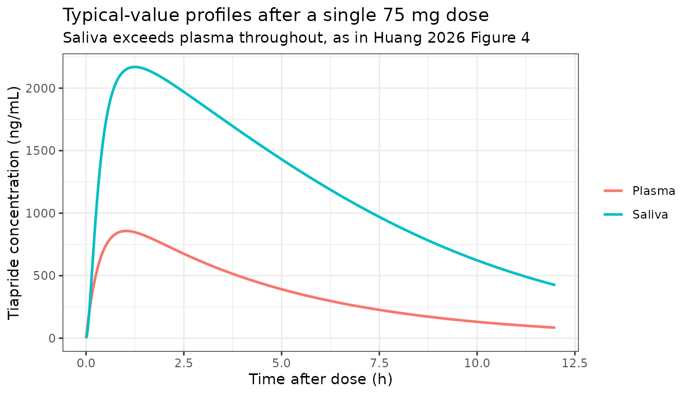
Saliva peaks later and higher than plasma, and decays in parallel with it once quasi steady state is reached – the qualitative shape of Figure 4B.
sal_peak_time <- sim_typ$time[which.max(sim_typ$Csaliva)]

c(plasma_tmax = tmax_cf, saliva_tmax = sal_peak_time,
  saliva_peak_ng_mL = 1000 * max(sim_typ$Csaliva))
#>       plasma_tmax       saliva_tmax saliva_peak_ng_mL
#>          1.025165          1.240000       2169.117858

stopifnot(
  # Saliva lags plasma: the transport is driven by Cc and the saliva state
  # needs a few of its own half-lives to catch the rising plasma curve.
  sal_peak_time > tmax_cf,
  # but only slightly, given the 6.7-minute saliva half-life.
  sal_peak_time - tmax_cf < 0.5,
  # Saliva above plasma from the peak onwards. NOT asserted before the peak:
  # the saliva compartment starts empty and needs a few of its own half-lives
  # to fill, so Csaliva is legitimately below Cc during the first minutes
  # after the dose. The paper's paired samples were all drawn at clinic
  # visits well past that window.
  all(sim_typ$Csaliva[post_peak] >= sim_typ$Cc[post_peak]),
  all(sim_typ$Csaliva >= 0)
)
Covariate effect of fat-free mass
ffm_grid <- seq(18, 50, by = 1)
cl_by_ffm <- cl_tv * (ffm_grid / 30.62)^ui$theta[["e_ffm_cl"]]

ggplot(data.frame(FFM = ffm_grid, CL = cl_by_ffm), aes(FFM, CL)) +
  geom_line(linewidth = 0.8) +
  geom_point(data = data.frame(FFM = 30.62, CL = cl_tv), size = 2.5) +
  labs(x = "Fat-free mass (kg)", y = "Apparent clearance CL/F (L/h)",
       title = "Equation 6: CL/F = 15.3 * (FFM/30.62)^0.553") +
  theme_bw()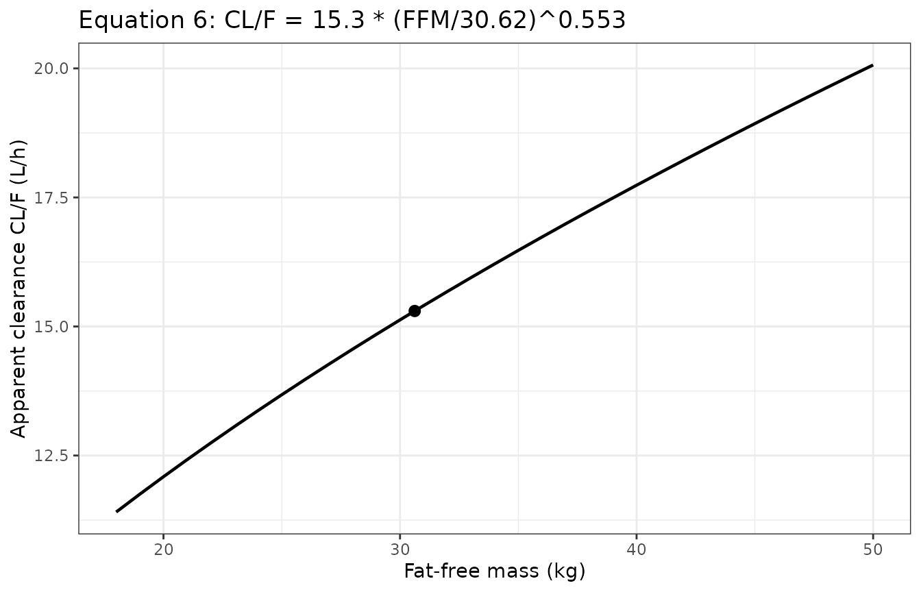
# Across the cohort IQR, clearance spans a factor of:
round((34.65 / 26.93)^ui$theta[["e_ffm_cl"]], 3)
#> [1] 1.15
Over the interquartile range of fat-free mass in the study population, apparent clearance varies by only about 14%, consistent with the modest exponent and its wide bootstrap confidence interval (0.277-0.771).
Assumptions and deviations
The saliva volume is assumed, not reported
This is the one assumed value in the model file, and it sits
directly under the saliva layer’s primary output. Read this section
before using Csaliva quantitatively.
Every other saliva parameter is printed: Vmax = 34.7
mg/h (Equation 8), Km = 762 ng/mL held constant (Equation
9), and K30 = 6.24 * (FFM/30.62)^0.38 * exp(eta) (Equation
10), with 30% IIV on K30 and 28.4% proportional residual error (Table
3). Those three constants fully determine the amount of drug in
the saliva compartment. Converting that amount to the observed saliva
concentration needs one more quantity – an apparent saliva
volume – and it appears nowhere in the paper: not in Tables 1-3, not in
Equations 1-10 (all ten were rendered from the PDF’s vector graphics and
read), not in any figure caption, and not in the Methods. In NONMEM this
would have been a $SCALE/S3 statement rather
than a $THETA, which is very likely why it never reached
the parameter table.
No other source holds it: the article (PMC13111164) has
no supplementary material and carries no data-availability or
supplementary-material statement. This is a reporting gap in the
publication itself.
Writing the quasi-steady-state form
Csaliva = Vmax * Cc / ((Km + Cc) * K30 * Vsaliva),
Vsaliva is the only unknown, and candidate recoveries span
more than threefold depending on which published quantity is used to pin
it:
| Basis for recovery | Implied Vsaliva
|
Disposition |
|---|---|---|
| Model median saliva / plasma at the Figure 4 VPC peak | 1.35 L | Adopted |
NONMEM’s default S3 = 1 (a unit-volume
compartment) |
1 L | Rejected – puts the low-concentration S/P near 7.3 against a reported mean of 2.3, the worst agreement with the paper’s own data of any candidate |
| Fitting the Figure 1 regressions to the saturating form | ~1.9 L | Rejected – the two regressions are not mutually consistent with a single saturating curve |
| The reported mean saliva:plasma ratio of 2.3 | ~3.2 L | Rejected – exact only in the low-concentration limit, and puts saliva about 35% below the Figure 4B median at the peak |
Sharing the central volume, as Nguyen_2026_linezolid
does |
5.77 L | Falsified – gives saliva below plasma, contradicting the paper’s central finding |
The adopted value and its provenance.
Vsaliva = 1.35 L was recovered by digitising Figure 4 at
500 dpi. At the roughly 2 h peak the model’s median plasma prediction is
about 790 ng/mL and its median saliva prediction about 2100 ng/mL;
substituting into the quasi-steady-state form gives
A_saliva = 34.7 x 0.790 / ((0.762 + 0.790) x 6.24) = 2.83
mg and hence Vsaliva = 1000 x 2.83 / 2100 = 1.35 L. The
value is annotated inline in ini() as figure-derived. This
follows the standing figure-digitisation policy for parameters available
only graphically, and was maintainer-ratified on
2026-09-21.
What this costs. Three caveats, in decreasing order of importance:
-
The Figure 4 peak is calibration, not validation.
Vsalivawas chosen to make the model reproduce that point, so agreement there is circular and is not claimed as a check anywhere in this vignette. The genuinely independent comparisons are the mean saliva:plasma ratio of 2.3 from the Discussion and the Figure 1 paired regressions, neither of which was used in the recovery; both are gated above. - The recovery is uncertain by roughly twofold. Applying the same algebra at trough times rather than at the peak yields about 2.4 L. The digitisation itself is good to perhaps +/- 25%, but the choice of anchor point matters more than the reading precision.
-
Vsalivacannot fix the shape. It scales the whole S/P curve uniformly, so it slides agreement between low and high concentrations without ever achieving both. The model’s S/P falls about threefold from 200 to 1700 ng/mL, whereas the Figure 1 paired regressions imply a milder decline. That is a property of the publishedKm= 762 ng/mL sitting inside the observed plasma range, and it would be present at anyVsaliva.
Anyone needing quantitatively reliable saliva predictions should
treat Csaliva as accurate to within a factor of about two,
use it in the high-concentration region where it agrees best with Figure
1, and ideally write to the corresponding authors (Xiaorong Yin,
sunnyxrr@126.com; Xuemei Wu,
wuxuemei@fjmu.edu.cn) for the scale statement. The plasma
layer carries none of this uncertainty.
Two saliva values differ between Table 3 and the Discussion
The Discussion states “the estimated K30 was 6.19 h-1” and “an IIV of 31.3% in K30”, where Table 3 and Equation 10 both print 6.24 1/h and 30%. The model follows Table 3 and Equation 10, on the standing rule that a printed equation and the final parameter table outrank a Discussion recollection. The difference is well inside the bootstrap interval (5.72-6.8 for K30) and moves no conclusion.
The saliva transport is encoded as driven, not depleting
The paper never writes the central compartment’s differential
equation, so whether the Michaelis-Menten term is subtracted from
central is a reconstruction. It is encoded as driven
(central is untouched) on the three grounds set out in the saliva
section above – the dashed arrow in Figure 2, the sequential fit with
plasma parameters held fixed, and the fact that the printed
Vmax is too large to be mass-conserving. The same
structural reading was maintainer-ratified for
Nguyen_2026_linezolid.R, the other saliva model in this
library. Were the term instead depleting, the plasma layer would no
longer reproduce Table 2 and the CL/F * AUC = dose identity
would fail by tens of percent, so this is not a fine distinction.
Much of the observed saliva data sits above the highest calibrator
The LC-MS/MS saliva assay was calibrated over 4-2000 ng/mL (Methods), but Figure 4B shows observed saliva concentrations reaching about 3900 ng/mL and a median above 2000 ng/mL at the peak. A substantial part of the saliva data the model was fitted to therefore lies above the calibrated range. The paper does not comment on this. It is a property of the source, not of the implementation, but it bears on how much weight the saliva layer will carry.
Interindividual variability scale
Table 2 heads the variability rows eta Ka (%),
eta CL/F (%) and eta Vd/F (%) – the eta itself
as a percentage – so they are read as omega * 100 and
encoded as omega^2. The paper prints no CV% column and no
control stream that would settle the convention independently. Read
instead as a log-normal CV%, the two small terms barely move (17.6%
-> 0.1745, 22.8% -> 0.2249) but Vd/F would fall from 0.843 to
0.7444. Given the 56% shrinkage on eta Vd/F and the
bootstrap interval spanning 30-133%, that term carries little
information either way.
Other assumptions
-
Fat-free mass equation. The paper does not state
how the FFM column was derived. For a 5-15 year old cohort the
Al-Sallami paediatric correction to the Janmahasatian adult formula is
the usual choice, and a user supplying
FFMshould compute it that way. The virtual cohort here draws FFM directly from a log-normal matched to the Table 1 median and IQR, as the paper did. -
Bioavailability. The study is oral-only, so
CL/FandVd/Fare apparent. NoFterm is reported and none is encoded. -
Units. The model works in mg / L / h, so
Ccis in mg/L; the paper reports ng/mL throughout and 1 mg/L = 1000 ng/mL. The additive residual 87.9 ng/mL is encoded as 0.0879 mg/L. - Dosing schedule for Figure 5. The paper says “simulated for 5 consecutive days” and plots 120-132 h, so the last dose is at t = 120 h with observation over the following 12 h and no further doses; that is what is reproduced.
-
PTA definition. The paper’s phrasing (“the
proportion of simulated steady-state peak concentration within the
therapeutic window of 560-2000 ng/mL”) is ambiguous, but only the
lower-bound reading
P(Cmax >= 560)reproduces the reported 97-98% values while also leaving room for the paper’s separate observation that the 100 mg regimens push more patients above 2000 ng/mL. Both quantities are tabulated above. -
Internal inconsistencies in the source. The
Discussion states
K30 = 6.19 1/hand an IIV of 31.3% where Table 3 gives 6.24 and 30%, and says the optimal regimen is “75 mg bid” where the Abstract, Results and Conclusions all say 75 mg tid. The tables and the majority text are taken as authoritative. Table 1 prints BSA in “cm2” and BMI in “kg cm2”, both of which are typographical errors for m^2 and kg/m^2.
Session information
#> R version 4.6.1 (2026-06-24)
#> Platform: x86_64-pc-linux-gnu
#> Running under: Ubuntu 24.04.5 LTS
#>
#> Matrix products: default
#> BLAS:   /usr/lib/x86_64-linux-gnu/openblas-pthread/libblas.so.3
#> LAPACK: /usr/lib/x86_64-linux-gnu/openblas-pthread/libopenblasp-r0.3.26.so;  LAPACK version 3.12.0
#>
#> locale:
#>  [1] LC_CTYPE=C.UTF-8       LC_NUMERIC=C           LC_TIME=C.UTF-8
#>  [4] LC_COLLATE=C.UTF-8     LC_MONETARY=C.UTF-8    LC_MESSAGES=C.UTF-8
#>  [7] LC_PAPER=C.UTF-8       LC_NAME=C              LC_ADDRESS=C
#> [10] LC_TELEPHONE=C         LC_MEASUREMENT=C.UTF-8 LC_IDENTIFICATION=C
#>
#> time zone: UTC
#> tzcode source: system (glibc)
#>
#> attached base packages:
#> [1] stats     graphics  grDevices utils     datasets  methods   base
#>
#> other attached packages:
#> [1] ggplot2_4.0.3         tidyr_1.3.2           dplyr_1.2.1
#> [4] PKNCA_0.12.1          rxode2_5.1.8          nlmixr2lib_0.3.2.9000
#>
#> loaded via a namespace (and not attached):
#>  [1] gtable_0.3.6        xfun_0.61           bslib_0.12.0
#>  [4] rxode2lincmt_0.1.0  lattice_0.22-9      vctrs_0.7.3
#>  [7] tools_4.6.1         generics_0.1.4      parallel_4.6.1
#> [10] tibble_3.3.1        symengine_0.2.13    pkgconfig_2.0.3
#> [13] data.table_1.18.6.1 checkmate_2.3.4     RColorBrewer_1.1-3
#> [16] S7_0.2.2            desc_1.4.3          lifecycle_1.0.5
#> [19] compiler_4.6.1      farver_2.1.2        textshaping_1.0.5
#> [22] fontawesome_0.5.3   htmltools_0.5.9     sys_3.4.3
#> [25] sass_0.4.10         yaml_2.3.12         pillar_1.11.1
#> [28] pkgdown_2.2.1       crayon_1.5.3        jquerylib_0.1.4
#> [31] whisker_0.4.1       openssl_2.4.2       cachem_1.1.0
#> [34] nlme_3.1-169        tidyselect_1.2.1    digest_0.6.39
#> [37] lotri_1.0.5         purrr_1.2.2         labeling_0.4.3
#> [40] rxode2ll_2.0.18     fastmap_1.2.0       grid_4.6.1
#> [43] cli_3.6.6           dparser_1.3.1-13    magrittr_2.0.5
#> [46] withr_3.0.3         scales_1.4.0        backports_1.5.1
#> [49] rmarkdown_2.32      otel_0.2.0          askpass_1.2.1
#> [52] ragg_1.5.2          memoise_2.0.1       evaluate_1.0.5
#> [55] knitr_1.52          rex_1.2.2           PreciseSums_0.7
#> [58] rlang_1.3.0         downlit_0.4.5       Rcpp_1.1.2
#> [61] glue_1.8.1          xml2_1.6.0          jsonlite_2.0.0
#> [64] R6_2.6.1            systemfonts_1.3.2   fs_2.1.0