Artemisinin + naphthoquine (Ali 2022)
Source:vignettes/articles/Ali_2022_artemisinin_naphthoquine.Rmd
Ali_2022_artemisinin_naphthoquine.RmdModel and source
Ali 2022 fitted two separate population PK models to the same patients, one for each component of the single-dose artemisinin-naphthoquine (ART-NQ) combination. Both are packaged:
-
Ali_2022_artemisinin: One-compartment population PK model for oral artemisinin given as a single dose of the fixed-dose artemisinin-naphthoquine combination to Tanzanian children (6 years and older) and adults with uncomplicated Plasmodium falciparum malaria (Ali 2022). Savic transit-compartment absorption (non-integer NN transit compartments and a separate first-order absorption rate ka into the central compartment), relative bioavailability fixed to 1 with between-subject variability, and allometric scaling by total body weight to a 55 kg reference (exponent 0.75 on CL/F, 1 on V/F). Naphthoquine from the same combination is a separately fitted model (Ali_2022_naphthoquine). -
Ali_2022_naphthoquine: Two-compartment population PK model for oral naphthoquine given as a single dose of the fixed-dose artemisinin-naphthoquine combination to Tanzanian children (6 years and older) and adults with uncomplicated Plasmodium falciparum malaria (Ali 2022). Savic transit-compartment absorption (non-integer NN transit compartments and a separate first-order absorption rate ka into the central compartment), relative bioavailability fixed to 1 with between-subject variability, and allometric scaling of CL/F by fat-free mass to a 45 kg reference (exponent 0.75) and of Q/F (exponent 0.75), Vc/F and Vp/F (exponent 1) by total body weight to a 55 kg reference. Artemisinin from the same combination is a separately fitted model (Ali_2022_artemisinin). - Citation: Ali AM, Gausi K, Jongo SA, Kassim KR, Mkindi C, Simon B, Mtoro AT, Juma OA, Lweno ON, Gwandu CH, Bakari BM, Mbaga TA, Milando FA, Hamad A, Shekalaghe SA, Abdulla S, Denti P, Penny MA (2022). Population Pharmacokinetics of Antimalarial Naphthoquine in Combination with Artemisinin in Tanzanian Children and Adults: Dose Optimization. Antimicrobial Agents and Chemotherapy 66(5):e01696-21. doi:10.1128/aac.01696-21.
- Article: https://doi.org/10.1128/aac.01696-21 (open access, PMC9112936)
Population
Ali 2022 enrolled 29 Tanzanian patients with uncomplicated Plasmodium falciparum malaria at the Bagamoyo Clinical Trial Unit in 2014, in the ART-NQ arm of a phase IV randomised study (NCT01930331). Patients were aged 6.0 to 56.0 years (median 13.1) and weighed 20 to 84 kg (median 32.0); 14 of 29 (48%) were female. Table 1 splits them into three age groups: 6-10 years (n = 12, median 20.0 kg), 11-17 years (n = 6, median 37.5 kg) and 18 years and older (n = 11, median 55.0 kg). Every patient received one oral dose of ART-NQ tablets (125 mg artemisinin + 50 mg naphthoquine each), about 20 mg/kg artemisinin and 8 mg/kg naphthoquine, rounded to whole tablets by weight band (Table 3). The achieved median doses were 18.5 mg/kg artemisinin and 7.4 mg/kg naphthoquine.
Artemisinin was sampled at 1, 2, 4, 8, 12 and 18 h after the dose. One slow absorber was excluded, leaving 28 patients and 174 samples. Naphthoquine was sampled at the same times and also on days 4, 7, 14, 21, 28 and 42, giving 363 concentrations from 29 patients.
The same information is available programmatically via
readModelDb("Ali_2022_naphthoquine")()$population.
Source trace
The per-parameter origin is recorded as an in-file comment next to
each ini() entry in
inst/modeldb/specificDrugs/Ali_2022_artemisinin.R and
inst/modeldb/specificDrugs/Ali_2022_naphthoquine.R. The
table below collects them in one place.
| Equation / parameter | Artemisinin | Naphthoquine | Source location |
|---|---|---|---|
lcl (CL/F, L/h) |
log(66.7) | log(44.2) | Table 2 |
lvc (V1/F, L) |
log(395) | log(647) | Table 2 |
lq (Q/F, L/h) |
n/a | log(601) | Table 2 |
lvp (Vp/F, L) |
n/a | log(19100) | Table 2 |
lka (1/h) |
log(2.11) | log(0.108) | Table 2 |
lmtt (h) |
log(0.987) | log(1.23) | Table 2 |
lnn (transit compartments) |
log(7.53) | log(5.42) | Table 2 |
lfdepot |
fixed(log(1)) | fixed(log(1)) | Table 2; Methods |
| allometric exponents |
e_wt_cl fixed 0.75, e_wt_vc fixed 1 |
e_ffm_cl and e_wt_q fixed 0.75,
e_wt_vc fixed 1 |
Methods; Table 2 footnote a |
| CL size descriptor | (WT/55)^0.75 | (FFM/45)^0.75 | Table 2 footnote a equations |
| Q size descriptor | n/a | (WT/55)^0.75 | Table 2 footnote a (‘all clearance and volumes … scaled using the body weight’ except naphthoquine CL) |
| V1, Vp size descriptor | (WT/55) | (WT/55) | Table 2 footnote a |
etalcl |
0.186^2 | 0.199^2 | Table 2 IIV; footnote d (%CV = sqrt(omega^2) x 100) |
etalka |
0.457^2 | 0.370^2 | Table 2 IIV |
etalmtt |
0.492^2 | 0.806^2 | Table 2 IIV |
etalfdepot |
0.411^2 | 0.327^2 | Table 2 IIV |
addSd (ng/mL) |
fixed(0.20) | 0.594 | Table 2; footnote c |
propSd |
0.307 | 0.251 | Table 2 |
Transit absorption into absorption compartment, then ka
to central |
yes | yes | Figure 1; Methods (reference 52, Savic 2007) |
d/dt(central), d/dt(peripheral1)
|
1-compartment | 2-compartment | Figure 1; Results |
Cc ~ add(addSd) + prop(propSd) |
yes | yes | Methods (‘combined additive and proportional error model’) |
Virtual cohorts
The observed data are not public. Two virtual cohorts are used.
- A study-like cohort of three age groups, 100 patients each, whose body weight and body mass index are drawn log-normally around the Table 1 median and interquartile range of each group, with each group’s Table 1 sex ratio.
- A weight-band cohort for Figure 4, with body weight uniform over the 16-80 kg range plotted there, and a separate cohort reproducing the efficacy target population (400 mg naphthoquine in patients weighing 47.8 +/- 4.3 kg, Methods ‘Simulations’).
Naphthoquine clearance scales with fat-free mass, which Ali 2022 derived “for males and females separately” without printing the equation. The Janmahasatian 2005 equations are used here, computed from body weight, body mass index and sex.
rxode2::rxSetSeed(20220425)
set.seed(20220425)

ffm_janmahasatian <- function(wt, bmi, sexf) {
  ifelse(sexf == 1, 9270 * wt / (8780 + 244 * bmi), 9270 * wt / (6680 + 216 * bmi))
}

# Table 3 'Current dose regimen' bands (naphthoquine / artemisinin in mg).
band_dose <- function(wt, optimised = FALSE) {
  nq <- dplyr::case_when(
    wt < 21 ~ 150,
    wt < 33 ~ 200,
    wt < 50 ~ 300,
    optimised & wt >= 70 ~ 500,
    TRUE ~ 400
  )
  list(nq = nq, art = nq * 2.5)
}

# Table 1 medians and IQRs per age group; sdlog = log(Q3 / Q1) / 1.349.
groups <- tibble::tribble(
  ~agegrp,     ~n,  ~wt_med, ~wt_q1, ~wt_q3, ~bmi_med, ~bmi_q1, ~bmi_q3, ~pfemale,
  "6-10 yr",   100, 20.0,    20.0,   24.5,   14.7,     14.1,    15.5,    9 / 12,
  "11-17 yr",  100, 37.5,    26.0,   48.0,   15.8,     14.1,    20.5,    2 / 6,
  ">= 18 yr",  100, 55.0,    51.0,   64.0,   20.4,     19.0,    25.3,    3 / 11
)

make_group <- function(g, id_offset) {
  n <- g$n
  tibble(
    id = id_offset + seq_len(n),
    agegrp = g$agegrp,
    WT = pmin(pmax(rlnorm(n, log(g$wt_med), log(g$wt_q3 / g$wt_q1) / 1.349), 18), 90),
    BMI = rlnorm(n, log(g$bmi_med), log(g$bmi_q3 / g$bmi_q1) / 1.349),
    SEXF = rbinom(n, 1, g$pfemale)
  )
}

study <- dplyr::bind_rows(lapply(seq_len(nrow(groups)), function(i) {
  make_group(groups[i, ], id_offset = (i - 1L) * 100L)
})) |>
  mutate(
    FFM = ffm_janmahasatian(WT, BMI, SEXF),
    nq_mg = band_dose(WT)$nq,
    art_mg = band_dose(WT)$art,
    agegrp = factor(agegrp, levels = groups$agegrp)
  )
stopifnot(!anyDuplicated(study$id))

study |>
  group_by(agegrp) |>
  summarise(
    n = n(),
    `median WT (kg)` = median(WT),
    `median FFM (kg)` = median(FFM),
    `median ART dose (mg/kg)` = median(art_mg / WT),
    `median NQ dose (mg/kg)` = median(nq_mg / WT)
  ) |>
knitr::kable(digits = 1, caption = "Study-like virtual cohort.")| agegrp | n | median WT (kg) | median FFM (kg) | median ART dose (mg/kg) | median NQ dose (mg/kg) |
|---|---|---|---|---|---|
| 6-10 yr | 100 | 20.0 | 16.5 | 20.8 | 8.3 |
| 11-17 yr | 100 | 37.3 | 30.8 | 18.2 | 7.3 |
| >= 18 yr | 100 | 54.1 | 45.1 | 16.4 | 6.6 |
Table 1 reports median doses of 18.8 / 18.7 / 16.9 mg/kg artemisinin and 7.5 / 7.5 / 6.8 mg/kg naphthoquine by age group. The weight-band doses of the virtual cohort are within about 11% of these, with the same fall in mg/kg dose from children to adults.
make_events <- function(cohort, dose_col, obs_times) {
  dose <- cohort |>
    transmute(id, time = 0, amt = .data[[dose_col]], evid = 1L, cmt = "depot",
              WT, FFM, agegrp)
  obs <- tidyr::crossing(cohort |> select(id, WT, FFM, agegrp), time = obs_times) |>
    mutate(amt = 0, evid = 0L, cmt = "central")
  bind_rows(dose, obs) |> arrange(id, time, desc(evid)) |> as.data.frame()
}

times_art <- seq(0, 24, by = 0.25)
times_nq <- sort(unique(c(seq(0, 48, by = 0.5), seq(52, 1008, by = 8), 168, 336, 504, 672, 1000)))

ev_art <- make_events(study, "art_mg", times_art)
ev_nq <- make_events(study, "nq_mg", times_nq)
Simulation
mod_art <- readModelDb("Ali_2022_artemisinin")
mod_nq <- readModelDb("Ali_2022_naphthoquine")

sim_art <- rxode2::rxSolve(mod_art, events = ev_art, keep = c("agegrp", "WT")) |>
  as.data.frame()
#> ℹ parameter labels from comments will be replaced by 'label()'
sim_nq <- rxode2::rxSolve(mod_nq, events = ev_nq, keep = c("agegrp", "WT", "FFM")) |>
  as.data.frame()
#> ℹ parameter labels from comments will be replaced by 'label()'

# An all-zero profile would mean the transit() input never fired.
stopifnot(max(sim_art$Cc) > 100, max(sim_nq$Cc) > 1)
Mass balance of the transit absorption
With F = 1 (typical value), the whole dose must reach the systemic
circulation, so AUC(0-inf) * CL / dose must equal 1 for
both drugs.
tv_ev <- function(amt, tmax, by) {
  rbind(
    data.frame(id = 1, time = 0, amt = amt, evid = 1L, cmt = "depot"),
    data.frame(id = 1, time = seq(0, tmax, by = by), amt = 0, evid = 0L, cmt = "central")
  ) |> mutate(WT = 55, FFM = 45)
}
trap <- function(t, y) sum(diff(t) * (head(y, -1) + tail(y, -1)) / 2)

tv_art <- rxode2::rxSolve(rxode2::zeroRe(mod_art), events = tv_ev(1000, 72, 0.01))
#> ℹ parameter labels from comments will be replaced by 'label()'
#> ℹ omega/sigma items treated as zero: 'etalcl', 'etalka', 'etalmtt', 'etalfdepot'
tv_nq <- rxode2::rxSolve(rxode2::zeroRe(mod_nq), events = tv_ev(400, 20000, 0.5))
#> ℹ parameter labels from comments will be replaced by 'label()'
#> ℹ omega/sigma items treated as zero: 'etalcl', 'etalka', 'etalmtt', 'etalfdepot'
mb <- c(
  artemisinin = trap(tv_art$time, tv_art$Cc) * 66.7 / (1000 * 1000),
  naphthoquine = trap(tv_nq$time, tv_nq$Cc) * 44.2 / (400 * 1000)
)
mb
#>  artemisinin naphthoquine
#>    0.9999933    0.9999996
# Deterministic typical-value solve: only trapezoid and truncation error.
stopifnot(all(abs(mb - 1) < 0.01))
Replicate published figures
Figure 2: artemisinin VPC
# Observed medians read by the maintainers from Figure 2 of Ali 2022 (solid
# red line); approximate, for visual orientation only.
fig2_obs <- data.frame(time = c(1, 2, 4, 8, 12, 18),
                       Cc = c(520, 1300, 1950, 800, 370, 120))

vpc_art <- sim_art |>
  filter(time > 0, time <= 19) |>
  group_by(time) |>
  summarise(Q05 = quantile(Cc, 0.05), Q50 = median(Cc), Q95 = quantile(Cc, 0.95),
            .groups = "drop")

ggplot(vpc_art, aes(time, Q50)) +
  geom_ribbon(aes(ymin = Q05, ymax = Q95), fill = "steelblue", alpha = 0.25) +
  geom_line(colour = "steelblue4") +
  geom_point(data = fig2_obs, aes(time, Cc), colour = "red", shape = 1, size = 2.5) +
  scale_y_log10() +
  labs(x = "Time after dose (h)", y = "Artemisinin concentration (ng/mL)",
       caption = paste("Replicates Figure 2 of Ali 2022. Line and band: simulated",
                       "median and 90% interval;\nopen circles: observed medians",
                       "read from the published figure."))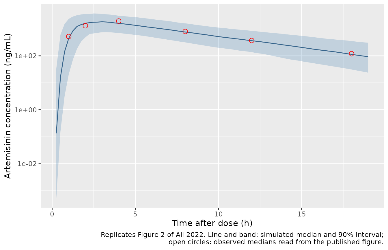
Figure 3: naphthoquine VPC
# Observed medians read by the maintainers from Figure 3 of Ali 2022.
fig3_obs <- data.frame(time = c(4, 12, 48, 168, 336, 504, 672, 1000),
                       Cc = c(55, 32, 20, 13, 8.5, 5, 3.5, 2.3))

vpc_nq <- sim_nq |>
  filter(time > 0) |>
  group_by(time) |>
  summarise(Q05 = quantile(Cc, 0.05), Q50 = median(Cc), Q95 = quantile(Cc, 0.95),
            .groups = "drop")

ggplot(vpc_nq, aes(time, Q50)) +
  geom_ribbon(aes(ymin = Q05, ymax = Q95), fill = "steelblue", alpha = 0.25) +
  geom_line(colour = "steelblue4") +
  geom_point(data = fig3_obs, aes(time, Cc), colour = "red", shape = 1, size = 2.5) +
  scale_y_log10() +
  labs(x = "Time after dose (h)", y = "Naphthoquine concentration (ng/mL)",
       caption = paste("Replicates Figure 3 of Ali 2022. Line and band: simulated",
                       "median and 90% interval;\nopen circles: observed medians",
                       "read from the published figure."))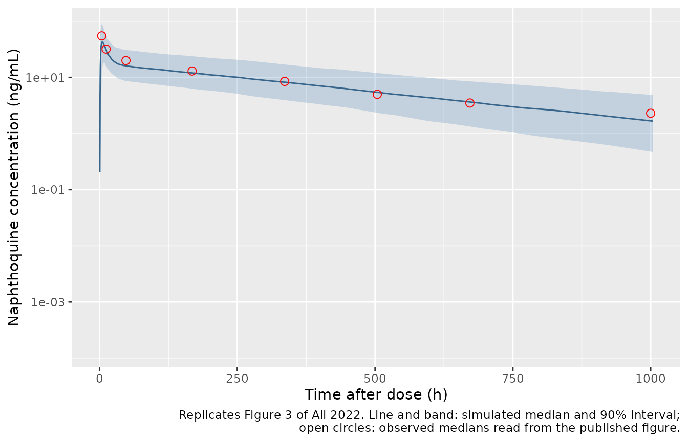
bind_rows(
  fig2_obs |> mutate(drug = "artemisinin") |>
    left_join(vpc_art |> select(time, sim = Q50), by = "time"),
  fig3_obs |> mutate(drug = "naphthoquine") |>
    left_join(vpc_nq |> select(time, sim = Q50), by = "time")
) |>
  mutate(ratio = sim / Cc) |>
  dplyr::rename("Drug" = drug, "Time (h)" = time,
                "Observed median, read from figure (ng/mL)" = Cc,
                "Simulated median (ng/mL)" = sim, "Simulated / observed" = ratio) |>
knitr::kable(digits = 2, caption = "Simulated median against the observed median of Figures 2 and 3.")| Time (h) | Observed median, read from figure (ng/mL) | Drug | Simulated median (ng/mL) | Simulated / observed |
|---|---|---|---|---|
| 1 | 520.0 | artemisinin | 445.65 | 0.86 |
| 2 | 1300.0 | artemisinin | 1613.25 | 1.24 |
| 4 | 1950.0 | artemisinin | 1599.25 | 0.82 |
| 8 | 800.0 | artemisinin | 762.94 | 0.95 |
| 12 | 370.0 | artemisinin | 364.88 | 0.99 |
| 18 | 120.0 | artemisinin | 113.40 | 0.94 |
| 4 | 55.0 | naphthoquine | 41.26 | 0.75 |
| 12 | 32.0 | naphthoquine | 30.96 | 0.97 |
| 48 | 20.0 | naphthoquine | 16.11 | 0.81 |
| 168 | 13.0 | naphthoquine | 12.01 | 0.92 |
| 336 | 8.5 | naphthoquine | 8.22 | 0.97 |
| 504 | 5.0 | naphthoquine | 5.43 | 1.09 |
| 672 | 3.5 | naphthoquine | 3.65 | 1.04 |
| 1000 | 2.3 | naphthoquine | 1.68 | 0.73 |
The simulated medians track the observed medians of both VPCs across the sampling window. The figure-read values are approximate and come from 28-29 patients, so this comparison is visual and is not used as a gate.
Figure 4 and the dose-optimisation claims
Ali 2022 simulated the day-7 naphthoquine concentration (the efficacy exposure) and Cmax (the safety exposure) across body weight under the current regimen and an optimised regimen that raises the dose to 500 mg naphthoquine from 70 kg. The efficacy target was the predicted day-7 concentration of patients weighing 47.8 +/- 4.3 kg given 400 mg: a median of 14.5 (IQR 11.7-18.6) ng/mL (Results ‘Simulations’). Patients of 70 kg or more on the current dose were reported to reach “on average a 30% lower day 7 concentration compared to a 48-kg reference patient” (Abstract).
The paper’s in silico population (1,333 African malaria patients) is not public. Body mass index for the weight-band cohort is interpolated from the Table 1 group medians (14.7, 15.8 and 20.4 kg/m^2 at 20, 37.5 and 55 kg), extended to 25 kg/m^2 at 80 kg, with half the patients female.
bmi_for_wt <- function(wt) {
  stats::approx(c(16, 20, 37.5, 55, 80), c(14.5, 14.7, 15.8, 20.4, 25), xout = wt, rule = 2)$y
}
make_wt_cohort <- function(n, wt, nq_mg, label, id_offset) {
  tibble(id = id_offset + seq_len(n), WT = wt, SEXF = rbinom(n, 1, 0.5)) |>
    mutate(BMI = bmi_for_wt(WT) * exp(rnorm(n, 0, 0.1)),
           FFM = ffm_janmahasatian(WT, BMI, SEXF),
           nq_mg = nq_mg, regimen = label)
}

wt_current <- runif(200, 16, 80)
wt_opt <- runif(200, 70, 80)
wt_target <- rnorm(200, 47.8, 4.3)
fig4 <- bind_rows(
  make_wt_cohort(200, wt_current, band_dose(wt_current)$nq, "Current", 0L),
  make_wt_cohort(200, wt_opt, band_dose(wt_opt, optimised = TRUE)$nq, "Optimised", 200L),
  make_wt_cohort(200, wt_target, 400, "Target (400 mg, 47.8 kg)", 400L)
)
stopifnot(!anyDuplicated(fig4$id))

ev_fig4 <- bind_rows(
  fig4 |> transmute(id, time = 0, amt = nq_mg, evid = 1L, cmt = "depot", WT, FFM, regimen),
  tidyr::crossing(fig4 |> select(id, WT, FFM, regimen),
                  time = c(seq(0, 24, by = 0.25), 168)) |>
    mutate(amt = 0, evid = 0L, cmt = "central")
) |> arrange(id, time, desc(evid)) |> as.data.frame()

sim4 <- rxode2::rxSolve(mod_nq, events = ev_fig4, keep = c("regimen", "WT")) |>
  as.data.frame()

expo <- sim4 |>
  group_by(id, regimen, WT) |>
  summarise(c7 = Cc[time == 168], cmax = max(Cc), .groups = "drop")
target <- expo |> filter(regimen == "Target (400 mg, 47.8 kg)")
target_q <- quantile(target$c7, c(0.05, 0.5, 0.95))

band_summary <- expo |>
  filter(regimen != "Target (400 mg, 47.8 kg)") |>
  mutate(wt_bin = floor(WT / 4) * 4 + 2) |>
  pivot_longer(c(c7, cmax), names_to = "metric", values_to = "value") |>
  group_by(regimen, metric, wt_bin) |>
  summarise(Q05 = quantile(value, 0.05), Q50 = median(value), Q95 = quantile(value, 0.95),
            .groups = "drop") |>
  mutate(metric = factor(metric, c("c7", "cmax"),
                         c("Day 7 concentration (ng/mL)", "Cmax (ng/mL)")))

hlines <- data.frame(
  metric = factor(c(rep("Day 7 concentration (ng/mL)", 3), "Cmax (ng/mL)"),
                  levels = levels(band_summary$metric)),
  y = c(unname(target_q), 156), lty = c("dashed", "solid", "dashed", "solid")
)

ggplot(band_summary, aes(wt_bin, Q50, colour = regimen, fill = regimen)) +
  geom_ribbon(aes(ymin = Q05, ymax = Q95), alpha = 0.2, colour = NA) +
  geom_line() +
  geom_hline(data = hlines, aes(yintercept = y, linetype = lty), colour = "purple") +
  scale_linetype_identity() +
  facet_wrap(~metric, ncol = 1, scales = "free_y") +
  labs(x = "Body weight (kg)", y = NULL, colour = "Regimen", fill = "Regimen",
       caption = paste("Replicates Figure 4 of Ali 2022 (4-kg bins). Purple lines:",
                       "efficacy target median and 5th/95th percentiles (top),\n",
                       "156 ng/mL safety Cmax (bottom)."))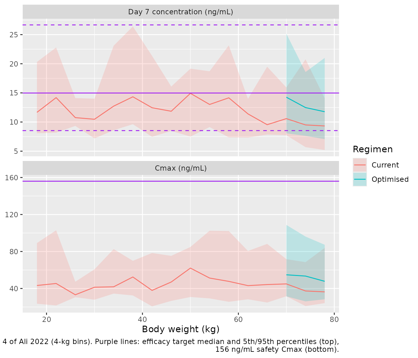
c7_ref <- median(target$c7)
c7_heavy <- median(expo$c7[expo$regimen == "Current" & expo$WT >= 70])
c7_heavy_opt <- median(expo$c7[expo$regimen == "Optimised"])
cmax_current <- median(expo$cmax[expo$regimen == "Current"])

tibble::tribble(
  ~quantity, ~simulated, ~published,
  "Target cohort median day-7 concentration (ng/mL)", c7_ref, 14.5,
  "Target cohort day-7 25th percentile (ng/mL)", unname(quantile(target$c7, 0.25)), 11.7,
  "Target cohort day-7 75th percentile (ng/mL)", unname(quantile(target$c7, 0.75)), 18.6,
  ">= 70 kg (current dose) median day 7 / target median", c7_heavy / c7_ref, 0.70,
  ">= 70 kg (500 mg) median day 7 / target median", c7_heavy_opt / c7_ref, NA,
  "Median Cmax across 16-80 kg, current dose (ng/mL)", cmax_current, NA
) |>
  dplyr::rename("Quantity" = quantity, "Simulated" = simulated, "Ali 2022" = published) |>
knitr::kable(digits = 2, caption = "Figure 4 claims: simulated against published.")| Quantity | Simulated | Ali 2022 |
|---|---|---|
| Target cohort median day-7 concentration (ng/mL) | 14.98 | 14.5 |
| Target cohort day-7 25th percentile (ng/mL) | 11.85 | 11.7 |
| Target cohort day-7 75th percentile (ng/mL) | 18.80 | 18.6 |
| >= 70 kg (current dose) median day 7 / target median | 0.64 | 0.7 |
| >= 70 kg (500 mg) median day 7 / target median | 0.83 | NA |
| Median Cmax across 16-80 kg, current dose (ng/mL) | 45.63 | NA |
stopifnot(
  # Paper-stated centre of the efficacy target. A mis-transcribed CL, V or
  # unit moves this by tens of percent.
  abs(c7_ref / 14.5 - 1) < 0.2,
  # 'on average a 30% lower day 7 concentration' for >= 70 kg.
  c7_heavy / c7_ref > 0.55, c7_heavy / c7_ref < 0.85,
  # Figure 4B: the median Cmax stays far below the 156 ng/mL safety cut-off.
  cmax_current > 25, cmax_current < 100
)
PKNCA validation
Ali 2022 reports no non-compartmental results, so the NCA below characterises the packaged models by age group for reference rather than comparing them with published values. Artemisinin is evaluated over 0-24 h; naphthoquine over the 42-day sampling window with AUC extrapolated to infinity.
run_nca <- function(sim, events, end) {
  conc <- sim[sim$time <= end, c("id", "time", "Cc", "agegrp")] |>
    filter(!is.na(Cc))
  conc <- bind_rows(conc, conc |> distinct(id, agegrp) |> mutate(time = 0, Cc = 0)) |>
    distinct(id, agegrp, time, .keep_all = TRUE) |>
    arrange(id, time)
  dose <- events |> filter(evid == 1) |> select(id, time, amt, agegrp)
  conc_obj <- PKNCA::PKNCAconc(conc, Cc ~ time | agegrp + id)
  dose_obj <- PKNCA::PKNCAdose(dose, amt ~ time | agegrp + id)
  intervals <- data.frame(start = 0, end = Inf, cmax = TRUE, tmax = TRUE,
                          aucinf.obs = TRUE, half.life = TRUE)
  PKNCA::pk.nca(PKNCA::PKNCAdata(conc_obj, dose_obj, intervals = intervals))
}

nca_art <- run_nca(sim_art, ev_art, 24)
nca_nq <- run_nca(sim_nq, ev_nq, 1008)

nca_tab <- function(res, drug) {
  as.data.frame(res$result) |>
    filter(PPTESTCD %in% c("cmax", "tmax", "aucinf.obs", "half.life")) |>
    group_by(agegrp, PPTESTCD) |>
    summarise(median = median(PPORRES, na.rm = TRUE), .groups = "drop") |>
    pivot_wider(names_from = PPTESTCD, values_from = median) |>
    mutate(drug = drug) |>
    select(drug, agegrp, cmax, tmax, aucinf.obs, half.life)
}

bind_rows(nca_tab(nca_art, "artemisinin"), nca_tab(nca_nq, "naphthoquine")) |>
  dplyr::rename("Drug" = drug, "Age group" = agegrp, "Cmax (ng/mL)" = cmax,
                "Tmax (h)" = tmax, "AUC0-inf (ng*h/mL)" = aucinf.obs,
                "t1/2 (h)" = half.life) |>
knitr::kable(digits = 1, caption = "Median simulated NCA parameters by age group.")| Drug | Age group | Cmax (ng/mL) | Tmax (h) | AUC0-inf (ng*h/mL) | t1/2 (h) |
|---|---|---|---|---|---|
| artemisinin | 6-10 yr | 2207.1 | 2.5 | 13970.4 | 3.2 |
| artemisinin | 11-17 yr | 1976.5 | 2.5 | 13988.8 | 3.8 |
| artemisinin | >= 18 yr | 1716.9 | 2.5 | 14210.3 | 4.2 |
| naphthoquine | 6-10 yr | 44.3 | 4.0 | 8332.5 | 261.1 |
| naphthoquine | 11-17 yr | 49.1 | 4.0 | 7939.4 | 292.8 |
| naphthoquine | >= 18 yr | 47.7 | 4.5 | 8111.3 | 333.3 |
Median AUC is similar across the three age groups for both drugs: the weight-band regimen gives adults a lower mg/kg dose than children (Table 1), which offsets their higher clearance. The exposure shortfall the paper addresses appears only at the top of the weight range, above the last band boundary at 50 kg (Figure 4).
Assumptions and deviations
-
Fat-free mass equation. Ali 2022 says fat-free mass
was “derived for males and females separately” (Methods, reference 55)
but does not print the equation. The vignette uses the Janmahasatian
2005 equations for all ages, computed from body weight, body mass index
and sex. Users of
Ali_2022_naphthoquinemust supply anFFMcolumn. - Fat-free-mass reference value. The Table 2 footnote equation normalises naphthoquine CL/F to an FFM of 45 kg, while the Abstract and Results quote the typical clearance at an FFM of 44.3 kg. The model uses 45 kg, the printed equation. It also reproduces the paper’s own rescaling to a 70 kg adult with FFM 56.1 kg (CL = 52.0 L/h printed; 52.1 L/h with 45 kg, 52.8 L/h with 44.3 kg). The choice changes typical clearance by 1.2%.
- Q/F at 70 kg. The Table 2 footnote rescales Q to 744 L/h for a 70 kg adult. Scaling 601 L/h by (70/55)^0.75, as the footnote’s statement that all clearances except naphthoquine CL are scaled by body weight implies, gives 720 L/h. No exponent or descriptor in the paper gives 744 L/h exactly, so the model follows the stated rule. The rescaled CL (52.0 L/h), V1 (823 L) and Vp (24,300 L) are reproduced.
-
Transit-chain convention. Both models use Savic’s
transit absorption with a non-integer number of transit compartments and
a separately estimated
kaout of the absorption compartment. The packaged models use rxode2’stransit(), whose transit rate constant is (NN + 1) / MTT, the Savic form. The paper does not state the convention, and with no published Tmax the choice cannot be checked against the paper. The NN / MTT alternative would change only the timing of absorption, not the exposure (AUC = F x dose / CL either way). - IIV scale. Table 2 footnote d defines the reported %CV as sqrt(omega^2) x 100, so omega^2 = (CV / 100)^2 is used rather than log(CV^2 + 1).
- Residual error. The paper describes a combined additive and proportional error model without saying whether the components are summed as variances or as standard deviations. The nlmixr2 default (variances summed) is used.
- Body-weight / FFM figure. The Results reports dOFV “-14.4 versus -23.2” for clearance scaled by fat-free mass versus body weight and calls FFM better, which is the reverse of what the printed numbers imply. This affects only the model-selection narrative; the final model’s descriptors are fixed by the Table 2 footnote equations.
- Virtual cohorts. The study cohorts draw weight and body mass index log-normally from the Table 1 medians and IQRs, with each age group’s sex ratio. The Figure 4 cohort uses a uniform 16-80 kg weight distribution and an interpolated body mass index, because the 1,333-patient in silico population the paper used is not public. Doses follow the Table 3 weight bands.
- Figure-read values. The observed medians overlaid on the Figure 2 and Figure 3 replications were read from the published figures by the maintainers and are approximate. They are not used in any assertion.
- Excluded artemisinin subject. The artemisinin model was fitted to 28 of the 29 patients; the paper excluded one slow absorber and does not report its characteristics.
- Errata. No correction notice for Ali 2022 was found in Europe PMC as of 2026-10-01.