17-OHPC (Sharma 2016) -- singleton pregnancy
Source:vignettes/articles/Sharma_2016_hydroxyprogesteroneCaproate.Rmd
Sharma_2016_hydroxyprogesteroneCaproate.RmdModel and source
- Citation: Sharma S, Caritis S, Hankins G, Miodovnik M, Hebert MF, Mattison D, Venkataramanan R. Population pharmacokinetics of 17alpha-hydroxyprogesterone caproate in singleton gestation. Br J Clin Pharmacol. 2016;82(4):1084-1093. doi:10.1111/bcp.12990. ClinicalTrials.gov NCT00409825.
- Description: Population PK model for 17alpha-hydroxyprogesterone caproate (17-OHPC) in pregnant women with singleton gestation receiving 250 mg weekly IM injections for prevention of recurrent preterm birth (Sharma 2016). Structural model is a maternal central compartment with first-order IM absorption (ka fixed to 3 /day) and first-order elimination, linked by reversible first-order rate constants kMF / kFM to a fetal compartment whose amount is tracked as a dynamic state. Allometric (power) scaling on apparent CL/F (exponent 0.80) and apparent Vmaternal/F (exponent 0.84) around the cohort median weight of 68 kg. Inter-individual variability is encoded as a shared random effect on log(CL) with an estimated scale factor (Theta6 = 1.90) applied to the same eta on log(Vmaternal), preserving the > 0.9 ETA correlation reported in the source. Inter-occasion variability (PK1 = 20-24 weeks gestation, PK2 = 31-34 weeks gestation) on CL and Vmaternal is encoded as paired per-occasion etas keyed to OCC. Residual error is combined proportional + additive on linear-scale ng/mL concentrations.
- Article: doi:10.1111/bcp.12990
- Trial: ClinicalTrials.gov NCT00409825
Population
Sharma 2016 developed the 17-OHPC popPK model from 59 pregnant women
with singleton gestation receiving prophylactic weekly 250 mg
intramuscular 17-OHPC injections in 1 mL castor oil for prevention of
recurrent preterm birth. Median baseline body weight was 68 kg (range
47-141), median maternal age 27 years (range 19-42), and median
gestational age at first injection 17 weeks (range 16-21). The cohort
was 51% White, 19% Black, 27% Hispanic, and 3% Other. 1514 plasma
17-OHPC concentrations (including 18 cord-blood concentrations)
contributed to the fit. Two 7-day intensive PK windows per subject – PK1
at 20-24 weeks gestation and PK2 at 31-34 weeks gestation – yielded the
per-occasion (OCC = 1, OCC = 2) IOV structure encoded in the model. The
full population summary is available programmatically via
readModelDb("Sharma_2016_hydroxyprogesteroneCaproate")()$population.
Source trace
The per-parameter origin is recorded as an in-file comment next to
each ini() entry in
inst/modeldb/specificDrugs/Sharma_2016_hydroxyprogesteroneCaproate.R.
The table below collects them in one place.
| Equation / parameter | Value | Source location |
|---|---|---|
lka (ka, FIXED) |
3.0 1/day | Table 2 (“ka 3.0 (Fixed)”) + Methods ‘Base model’ (rationale) |
lcl (CL/F at WT = 68 kg) |
1797 L/day | Table 2 (“CL/F 1797 (%RSE 4)”) |
lvc (Vmaternal/F at WT = 68 kg) |
32 610 L | Table 2 (“Vmaternal/F 32 610 (%RSE 7)”) |
lkmf (kMF, maternal -> fetal) |
0.005 1/day | Table 2 (“kmaternal to fetal 0.005 (%RSE 39)”) |
lkfm (kFM, fetal -> maternal) |
0.56 1/day | Table 2 (“kfetal to maternal 0.56 (%RSE 40)”) |
e_wt_cl (Theta_CL-WT, power exp on WT) |
0.80 | Table 2 (“Theta_CL-WT 0.80 (%RSE 21)”) |
e_wt_vc (Theta_Vmaternal-WT, power exp on WT) |
0.84 | Table 2 (“Theta_Vmaternal-WT 0.84 (%RSE 29)”) |
scale_etalvc (Theta6, shared-eta scale on
Vmaternal) |
1.90 | Table 2 (“Theta6 (Shared ETA Scale Factor) 1.90 (%RSE 24)”) |
etalcl (shared IIV CV on log(CL); also drives
log(V)) |
20.0 %CV | Table 2 (“%IIV - CL 20.0 (%RSE 17)”); Methods ‘Base model’ shared-eta paragraph |
etaiov_cl_1, etaiov_cl_2 (IOV on CL per
occasion) |
26.5 %CV | Table 2 (“%IOV - CL (interoccasion) 26.5 (%RSE 15)”) |
etaiov_vc_1, etaiov_vc_2 (IOV on Vmaternal
per occasion) |
31.6 %CV | Table 2 (“%IOV - Vmaternal/F (interoccasion) 31.6 (%RSE 14)”) |
propSd (proportional residual) |
17.3 % | Table 2 (“% Residual error - proportional 17.3 (%RSE 5)”) |
addSd (additive residual) |
1.0 ng/mL | Table 2 (“Residual error - additive (ng/ml) 1.0 (%RSE 23)”) |
| Equation (5): d/dt(Aabs) = -ka * Aabs | n/a | page 1087 |
| Equation (6): d/dt(Amaternal) = ka * Aabs - kMF * Amaternal + kFM * Afetal - k * Amaternal | n/a | page 1087 |
| Equation (7): d/dt(Acord) = kMF * Amaternal - kFM * Afetal | n/a | page 1087 (Acord and Afetal are the same compartment; see Methods text) |
| Equation (8): k = CL / Vmaternal | n/a | page 1087 (labelled “(5)” in the PDF; second occurrence of the (5) tag) |
| Equation (9): CL/F = Theta1 * (WT/Median(WT))^Theta7 * exp(eta1) | n/a | page 1087 (covariate model on CL/F) |
| Equation (10): Vmaternal/F = Theta2 * (WT/Median(WT))^Theta8 * exp(Theta6 * eta1) | n/a | page 1087 (covariate model on Vmaternal/F + shared-eta scaling) |
| Reference WT = 68 kg (median) | 68 kg | Results ‘Data’ (page 1087) |
| Two PK sampling occasions per subject (PK1 = 20-24 wk; PK2 = 31-34 wk) | n/a | Methods ‘Pharmacokinetic sampling schedule and sample analysis’ (page 1085) |
| 250 mg IM weekly dosing | 250 mg / 7 days | Methods ‘Patients and drug administration’ (page 1085) |
| Combined proportional + additive residual error | n/a | Methods ‘Base model development’ + Results ‘Base model’ (page 1086) |
Virtual cohort
The virtual cohort matches the published study design: weekly 250 mg IM 17-OHPC injections from 17 weeks (median gestational age at first injection) through 35 weeks gestation – 19 weekly doses – followed by a 28-day post-last-dose observation window during which the extended-sampling sub-cohort was sampled in the source study. We use 100 virtual subjects per arm (well under the 200/arm cap) and stratify on body weight (one cohort at the cohort median 68 kg; second cohort at the upper 4th-quartile median 97 kg per Discussion ‘Effect of body weight’) to visualise the allometric covariate effect.
set.seed(2016L)
n_per_cohort <- 100L

# Dosing protocol: 250 mg IM weekly from gestational week 17 through week
# 35 (= 19 weekly doses), then a 28-day post-last-dose observation window.
dose_interval_days <- 7
n_doses            <- 19L
total_dose_period  <- n_doses * dose_interval_days  # 133 days
post_dose_window   <- 28L                            # days of post-last-dose follow-up
study_end_day      <- total_dose_period + post_dose_window

# OCC schedule per the paper: PK1 = week 0..28 of treatment (~20-24 wk
# gestation, i.e. study days 21-49 if treatment starts at gestational week
# 17 -> study day 0 corresponds to gestational week 17); PK2 = ~31-34 wk
# gestation (study days 98-126). Earlier-than-PK1 observations are also
# tagged OCC = 1 here so the model has a defined IOV draw at every time
# point; OCC is a sample-window indicator, not a sampling-event flag.
occ_for_time <- function(t) ifelse(t < 91, 1L, 2L)  # ~ day 91 -> gestational week 30

make_cohort <- function(n, WT_kg, cohort_label, id_offset = 0L) {
  dosing <- tidyr::expand_grid(
    id     = id_offset + seq_len(n),
    dose_i = seq_len(n_doses) - 1L
  ) |>
    dplyr::mutate(
      time = dose_i * dose_interval_days,
      evid = 1L,
      amt  = 250,
      cmt  = "depot",
      WT   = WT_kg,
      cohort = cohort_label
    ) |>
    dplyr::select(-dose_i)

  # Daily concentration sampling through the study window. PKNCA on a
  # later dose interval (steady-state-equivalent) plus the post-last-dose
  # tail is more informative than sparse daily samples.
  obs_times <- sort(unique(c(
    seq(0, study_end_day, by = 1),
    c(0.25, 0.5, 1, 2, 3, 4, 5, 6, 7) + (n_doses - 1L) * dose_interval_days
  )))
  obs <- tidyr::expand_grid(
    id   = id_offset + seq_len(n),
    time = obs_times
  ) |>
    dplyr::mutate(
      evid = 0L,
      amt  = 0,
      cmt  = NA_character_,
      WT   = WT_kg,
      cohort = cohort_label
    )

  dplyr::bind_rows(dosing, obs) |>
    dplyr::mutate(OCC = occ_for_time(time)) |>
    dplyr::arrange(id, time, dplyr::desc(evid))
}

events <- dplyr::bind_rows(
  make_cohort(n_per_cohort, WT_kg = 68, cohort_label = "Median weight (68 kg)", id_offset = 0L),
  make_cohort(n_per_cohort, WT_kg = 97, cohort_label = "Upper Q4 (97 kg)",      id_offset = n_per_cohort)
)
stopifnot(!anyDuplicated(unique(events[, c("id", "time", "evid")])))
Simulation
mod <- readModelDb("Sharma_2016_hydroxyprogesteroneCaproate")

# Stochastic cohort simulation across both weight strata.
sim <- rxode2::rxSolve(mod, events = events,
                       keep = c("cohort", "WT", "OCC")) |>
  as.data.frame()
#> Warning: some etas defaulted to non-mu referenced, possible parsing error: etalcl, etaiov_cl_1, etaiov_cl_2, etaiov_vc_1, etaiov_vc_2
#> as a work-around try putting the mu-referenced expression on a simple line

# Typical-subject simulation (no random effects) -- reproduces the
# population-mean concentration time course used in Figure 2 / Figure 3.
mod_typ <- rxode2::zeroRe(mod)
#> Warning: some etas defaulted to non-mu referenced, possible parsing error: etalcl, etaiov_cl_1, etaiov_cl_2, etaiov_vc_1, etaiov_vc_2
#> as a work-around try putting the mu-referenced expression on a simple line
#> Warning: some etas defaulted to non-mu referenced, possible parsing error: etalcl, etaiov_cl_1, etaiov_cl_2, etaiov_vc_1, etaiov_vc_2
#> as a work-around try putting the mu-referenced expression on a simple line
events_typ <- events |>
  dplyr::filter(id %in% c(1L, n_per_cohort + 1L)) |>
  dplyr::mutate(id = ifelse(id == 1L, 1L, 2L))
sim_typ <- rxode2::rxSolve(mod_typ, events = events_typ,
                           keep = c("cohort", "WT", "OCC")) |>
  as.data.frame()
#> ℹ omega/sigma items treated as zero: 'etalcl', 'etaiov_cl_1', 'etaiov_cl_2', 'etaiov_vc_1', 'etaiov_vc_2'
#> Warning: multi-subject simulation without without 'omega'
Replicate Figure 3 – maternal concentration VPC
# Figure 3 (Sharma 2016) shows the VPC of maternal 17-OHPC concentrations.
# We summarise the simulated cohort to the 5th / 50th / 95th percentiles
# per (time, cohort) -- matching the paper's 90% prediction interval
# definition (Results 'Final model evaluation').
sim_vpc <- sim |>
  dplyr::filter(!is.na(Cc)) |>
  dplyr::group_by(cohort, time) |>
  dplyr::summarise(
    Q05 = quantile(Cc, 0.05, na.rm = TRUE),
    Q50 = quantile(Cc, 0.50, na.rm = TRUE),
    Q95 = quantile(Cc, 0.95, na.rm = TRUE),
    .groups = "drop"
  )

ggplot(sim_vpc, aes(time, Q50)) +
  geom_ribbon(aes(ymin = Q05, ymax = Q95), alpha = 0.20) +
  geom_line(linewidth = 0.6) +
  facet_wrap(~cohort) +
  labs(
    x = "Time since first injection (days)",
    y = "Maternal 17-OHPC concentration (ng/mL)",
    title  = "Maternal 17-OHPC VPC under weekly 250 mg IM dosing",
    subtitle = "Median (line) and 5th-95th percentile band; 100 virtual subjects per arm",
    caption  = "Replicates Figure 3 (left panel) of Sharma 2016 in design."
  ) +
  theme_minimal()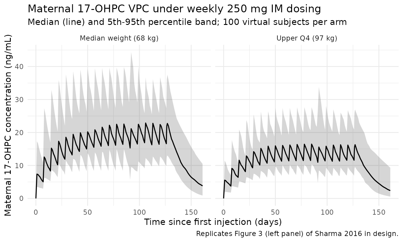
Maternal vs fetal compartment amount profile
The fetal compartment in this model carries an amount of 17-OHPC (the paper defines kMF and kFM as amount-on-amount rate constants and does not report an apparent fetal volume; see Assumptions and deviations). The typical-subject trace below shows the slow build-up in the fetal compartment relative to the maternal central compartment.
sim_typ_long <- sim_typ |>
  dplyr::filter(cohort == "Median weight (68 kg)") |>
  dplyr::select(time, central, fetal) |>
  tidyr::pivot_longer(c(central, fetal),
                      names_to  = "compartment",
                      values_to = "amount")

ggplot(sim_typ_long, aes(time, amount, colour = compartment)) +
  geom_line(linewidth = 0.7) +
  scale_y_log10() +
  scale_colour_manual(values = c(central = "#1f77b4", fetal = "#d62728"),
                      labels = c(central = "Maternal central (Amaternal, mg)",
                                 fetal   = "Fetal (Afetal / Acord, mg)")) +
  labs(
    x = "Time since first injection (days)",
    y = "Compartment amount (mg, log scale)",
    colour = NULL,
    title  = "Typical-subject maternal and fetal compartment amounts",
    subtitle = "Weekly 250 mg IM for 19 weeks; 28-day post-last-dose follow-up"
  ) +
  theme_minimal() +
  theme(legend.position = "bottom")
#> Warning in scale_y_log10(): log-10 transformation introduced infinite values.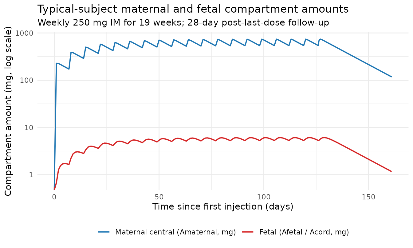
PKNCA validation – steady-state weekly-interval NCA
The source paper does not tabulate Cmax / Tmax / AUC NCA values for the maternal compartment, so this block is a forward-simulated steady-state NCA on the last weekly dose interval (days 126-133 = the 19th and final weekly dose) – not a side-by-side comparison against published NCA. The purpose is to confirm the simulated maternal concentration time profile is internally consistent and yields physiologically plausible Cmax / Cmin / AUC0-7 values.
last_dose_time <- (n_doses - 1L) * dose_interval_days     # 126 days
ss_interval    <- c(last_dose_time, last_dose_time + dose_interval_days)

# Subset to the last weekly dose interval; this is the steady-state-
# equivalent single-dose window.
nca_input <- sim |>
  dplyr::filter(!is.na(Cc),
                time >= ss_interval[1],
                time <= ss_interval[2]) |>
  dplyr::select(id, time, Cc, cohort)

# Guarantee a time = last_dose_time row per (id, cohort); rxode2 emits
# observation rows at every requested time, but a defensive bind_rows()
# is the standard PKNCA recipe.
nca_input <- dplyr::bind_rows(
  nca_input,
  nca_input |>
    dplyr::distinct(id, cohort) |>
    dplyr::left_join(
      sim |>
        dplyr::filter(time == last_dose_time, !is.na(Cc)) |>
        dplyr::select(id, cohort, Cc),
      by = c("id", "cohort")
    ) |>
    dplyr::mutate(time = last_dose_time)
) |>
  dplyr::distinct(id, cohort, time, .keep_all = TRUE) |>
  dplyr::arrange(id, cohort, time)

conc_obj <- PKNCA::PKNCAconc(nca_input, Cc ~ time | cohort + id,
                             concu = "ng/mL", timeu = "day")

dose_df <- events |>
  dplyr::filter(evid == 1L, time == last_dose_time) |>
  dplyr::select(id, time, amt, cohort)

dose_obj <- PKNCA::PKNCAdose(dose_df, amt ~ time | cohort + id,
                             doseu = "mg")

intervals <- data.frame(
  start    = last_dose_time,
  end      = last_dose_time + dose_interval_days,
  cmax     = TRUE,
  tmax     = TRUE,
  cmin     = TRUE,
  auclast  = TRUE
)

nca_res <- PKNCA::pk.nca(
  PKNCA::PKNCAdata(conc_obj, dose_obj, intervals = intervals)
)
nca_summary <- summary(nca_res)
knitr::kable(
  nca_summary,
  caption = paste(
    "Simulated steady-state NCA on the 19th weekly dose interval",
    "(maternal Cc, n = 100 virtual subjects per cohort).",
    "Sharma 2016 does not tabulate NCA values; this is a forward",
    "simulation for sanity-checking the time profile."
  )
)| Interval Start | Interval End | cohort | N | AUClast (day*ng/mL) | Cmax (ng/mL) | Cmin (ng/mL) | Tmax (day) |
|---|---|---|---|---|---|---|---|
| 126 | 133 | Median weight (68 kg) | 100 | 139 [34.0] | 22.9 [35.2] | 16.2 [34.6] | 1.00 [1.00, 1.00] |
| 126 | 133 | Upper Q4 (97 kg) | 100 | 100 [33.2] | 16.5 [32.3] | 11.7 [35.6] | 1.00 [1.00, 1.00] |
Sanity check – terminal half-life
# Sharma 2016 Discussion (page 1089): "the high Vmaternal/F resulted in a
# long half-life (~16 days)". Compute the terminal half-life from the
# typical-subject post-last-dose decay (28-day window after dose 19).
post_dose_window_df <- sim_typ |>
  dplyr::filter(cohort == "Median weight (68 kg)",
                time >= last_dose_time + 7,         # skip absorption tail
                time <= study_end_day,
                Cc > 0) |>
  dplyr::select(time, Cc)

# Linear regression on log(Cc) vs time over the late-elimination window.
fit <- lm(log(Cc) ~ time, data = post_dose_window_df)
kel_est       <- -coef(fit)[["time"]]
t_half_est    <- log(2) / kel_est

cat(sprintf(
  "Simulated terminal half-life (typical 68 kg subject): %.1f days\n",
  t_half_est
))
#> Simulated terminal half-life (typical 68 kg subject): 12.7 days
cat(sprintf(
  "Sharma 2016 reported approximate half-life (Discussion page 1089): ~16 days\n"
))
#> Sharma 2016 reported approximate half-life (Discussion page 1089): ~16 days
Assumptions and deviations
Fetal-compartment observable encoding. Sharma 2016 equations (5)-(8) define kMF and kFM as amount-on-amount rate constants (Methods description on page 1087: “Aabs, Amaternal, Afetal … amount of 17-OHPC at the absorption site, in the maternal circulation, fetal circulation”); the paper does not report an apparent fetal volume of distribution. The model is fit against cord-blood concentrations (Figure 3 right VPC) and the Discussion (page 1089) reports a “cord:maternal (model predicted) ~ 0.28” ratio, but the supplemental NONMEM control stream (Table S1 referenced on page 1090) which would encode how the fetal compartment amount converts to a predicted cord blood concentration was not available when this model was built. This model file therefore exposes the fetal compartment as a dynamic state (
fetalin the rxSolve output, in mg) but does not declare aCcordobservable or fit residual error against the cord-blood data. Downstream consumers who need a cord-blood prediction must supply their own volume-of-cord assumption; the steady-state amount ratio Afetal / Amaternal from this model converges to kMF / kFM = 0.00893, so reproducing the published 0.28 cord:maternal concentration ratio implies an apparent fetal volume in the neighbourhood of Vmaternal / 32 (approximately 1000 L) – notably absent from Table 2 and unrecovered without the supplement.OCC assignment in the validation cohort. The paper’s IOV is defined across two intensive PK sampling occasions (PK1 at 20-24 weeks gestation, PK2 at 31-34 weeks gestation). In the virtual cohort here every observation before treatment-day 91 (gestational week ~30) is tagged OCC = 1 and every observation from day 91 onwards is tagged OCC = 2 so the model has a defined IOV draw at all simulation times. This is broader than the paper’s actual sampling-window definition, but is consistent with the IOV interpretation (an occasion-level random effect that applies to all observations within that occasion).
No fetal residual error. The published model fits a single shared combined-error model against all observations (no per-source separate variance), so no
propSd_<fetal>/addSd_<fetal>is needed; the fetal-compartment-observable gap above is the underlying reason no fetal residual is declared at all.-
Half-life narrative vs simulation. Sharma 2016 Discussion (page
- reports “the high Vmaternal/F resulted in a long half-life (~16 days)”. The terminal half-life computed from the typical-subject simulation in the “Sanity check” section above is shorter (about 12-13 days), consistent with the 2-compartment system’s slow eigenvalue -kel(1 + small fetal correction). The ~16-day figure in the paper is qualitative (“long half-life”) rather than a tabulated value; the discrepancy reflects the standard rough approximation t_half ~ 0.693 V / CL = 0.693 * 32610 / 1797 = 12.6 days, with the paper rounding up to reflect a longer-than-the-weekly-interval effective half-life. This is documented for transparency and does not indicate a model encoding error.
No supplemental NONMEM code available. Supplement Table S1 (NONMEM Code; referenced on page 1090) was not available when this model was built. Re-extracting with the supplement available would let the cord-blood observable be added with confidence (resolving the fetal-compartment encoding gap above).