SNB-101 nanoparticle irinotecan and SN-38 (Park 2025)
Source:vignettes/articles/Park_2025_SNB101.Rmd
Park_2025_SNB101.RmdModel and source
- Citation: Park J, Bae SH, Jeon S, Park YH, Lee DC, Han S. Model-based prediction of nanoparticle and dissolved form ratios using total concentration data: a case study of SNB-101. Front Pharmacol. 2025;16:1556618. doi:10.3389/fphar.2025.1556618. PMCID: PMC12408558. Parameter values from Table 2; model structure and the fixed S-irinotecan variances from the NONMEM control stream in Supplementary Material 1. The fixed S-irinotecan parameters are from Minichmayr IK, Karlsson MO, Jonsson S. Pharm Res. 2021;38:593-605 (doi:10.1007/s11095-021-03024-w), as cited by the source.
- Description: Eleven-compartment population PK model for SNB-101, a
polymeric nanoparticle co-encapsulating irinotecan and SN-38 (about 1:1
molar), in adults with advanced solid tumours (Park 2025, phase I, N =
21). Each analyte is split into a nanoparticle (NP,
_npstates) and a dissolved (S, unsuffixed states) form fitted to total concentrations: NP-irinotecan (two compartments) releases into S-irinotecan (three compartments, parameters fixed from Minichmayr 2021) at krel; NP-SN-38 shares the NP-irinotecan volumes and distribution clearance and releases into S-SN-38 (two compartments) at krel_sn38; 3% of S-irinotecan clearance forms S-SN-38; all S-SN-38 clearance forms SN-38 glucuronide (central compartment with first-order clearance and a second, one-way first-order loss at Q6 into a peripheral compartment that does not return, as in the published control stream). Release is the only loss of each NP form. Amounts are in umol and concentrations in nmol/L. The NP:S split of each dose (irinotecan 0.15:0.85, SN-38 0.98:0.02) is applied in the dosing records, not in the model. - Article: https://doi.org/10.3389/fphar.2025.1556618 (open access, PMC12408558); the NONMEM control stream of the final model is Supplementary Material 1.
SNB-101 is a polymeric nanoparticle (mean size about 110 nm) that carries irinotecan and its active metabolite SN-38 at about a 1:1 molar ratio. Only total (nanoparticle + dissolved) plasma concentrations were measured in the phase I trial. The model separates each analyte into a nanoparticle (NP) form and a dissolved (S) form by fixing the disposition of S-irinotecan to a published model (Minichmayr 2021) and letting the data identify the rest:
- NP-irinotecan (two compartments) releases into S-irinotecan (three
compartments, fixed) at
krel; release is its only loss. - NP-SN-38 shares the NP-irinotecan central and peripheral volumes and
intercompartmental clearance, and releases into S-SN-38 (two
compartments) at
krel_sn38. - 3% (molar) of S-irinotecan clearance forms S-SN-38; all S-SN-38 clearance forms SN-38 glucuronide (SN-38G). SN-38G leaves its central compartment by clearance CL3 and by a one-way transfer Q6 into a peripheral compartment that does not return (see “SN-38G peripheral compartment” below).
- The observed analytes are total irinotecan (
Cc), total SN-38 (Cc_sn38) and SN-38G (Cc_sn38g), each with a proportional residual error. The form-specific concentrationsCc_np,Cc_dissolved,Cc_sn38_npandCc_sn38_dissolvedare model predictions only.
The model works in molar units (amounts in umol, concentrations in nmol/L), so the irinotecan -> SN-38 -> SN-38G conversions need no weight ratio. The NP:S composition of the drug product – irinotecan 0.15:0.85 and SN-38 0.98:0.02 – was put into the dosing records of the source dataset, and it is applied the same way here: each SNB-101 dose is four records.
Population
Twenty-one adults with advanced solid tumours refractory to, or without, standard therapy (ECOG 0-1, no prior topoisomerase I inhibitor) received a single intravenous dose of SNB-101 in Cycle 1 of the phase I trial NCT04640480, in seven escalation cohorts of 1, 1, 1, 5, 7, 3 and 3 patients (5-50 mg/m^2 as SN-38 with 8-80 mg/m^2 irinotecan; 14 men and 7 women; cohort mean ages 58-65 years and weights 68-75 kg; Park 2025 Table 1). Plasma was sampled at 0, 0.5, 1, 2, 4, 6, 8, 10, 12, 24, 36, 48, 72, 96, 120, 144 and 169.5 h. No covariate was retained.
Source trace
| Model element | Value | Source |
|---|---|---|
lcl (CL1, S-irinotecan) |
29.7 L/h | Table 2; $THETA(1)
|
lvc_np (V1 = V6) |
54.4 L | Table 2; $PK V6 = V1
|
lvp_np (V2 = V7) |
287 L | Table 2; $PK V7 = V2
|
lq_np (Q1 = Q4) |
6.45 L/h | Table 2; $PK Q4 = Q1
|
lkrel (k13) |
64.4 1/h | Table 2 |
lvc, lvp, lvp2 (V3, V4,
V5) |
68.6, 67.2, 127 L, fixed | Table 2 (‘FIX’); Minichmayr 2021 |
lq, lq2 (Q2, Q3) |
114, 9.89 L/h, fixed | Table 2 (‘FIX’); Minichmayr 2021 |
fm_sn38 |
0.03, fixed | Methods 2.2; $PK K38 = CL1*0.03/V3
|
lkrel_sn38 (k68) |
0.712 1/h | Table 2 |
lvc_sn38 (V8) |
40.3 L | Table 2 |
lvp_sn38 (V9 = V11) |
491 L | Table 2; $PK V11 = V9
|
lq_sn38 (Q5) |
121 L/h | Table 2 |
lcl_sn38 (CL2) |
167 L/h | Table 2; FMS = 1 FIX routes all of it to SN-38G |
lcl_sn38g, lq_sn38g,
lvc_sn38g (CL3, Q6, V10) |
16.9 L/h, 11.3 L/h, 7.84 L | Table 2 |
etalcl, etalvc_np,
etalvp_np
|
34.7%, 40.9%, 94.5% CV | Table 2, omega^2 = log(1 + CV^2)
|
etalvc … etalq2 (fixed) |
0.0233, 0.0258, 0.0813, 0.555, 0.219 |
$OMEGA 6-10 (Table 2: 15.4%, 16.2%, 29.1%, 86.1%,
49.5%) |
etalkrel_sn38, etalcl_sn38
|
39.6%, 44.9% CV | Table 2 |
etalcl_sn38g, etalvc_sn38g
|
115.9%, 122.1% CV | Table 2 |
propSd, propSd_sn38,
propSd_sn38g
|
0.21, 0.416, 0.308 | Table 2 (PROP1-3) |
| ODEs | 11 compartments | Supplement $DES (followed where it differs from Figure
2, see below) |
| Observations | NP + S totals; nmol/L | Supplement $ERROR (IND 1-3),
S = V/1000
|
| Dose split | irinotecan 0.15:0.85, SN-38 0.98:0.02 | Methods 2.2 |
The Table 2 BSV column is sqrt(exp(omega^2) - 1): the
five fixed S-irinotecan variances in $OMEGA reproduce the
printed percentages exactly (for example
sqrt(exp(0.0233) - 1) = 15.4%), so the estimated ones are
converted back the same way.
Dosing helper
Doses are given as mg/m^2 of SN-38 and of irinotecan. The helper converts them to umol and splits each into its NP and S records. Two quantities the paper does not print are set from Table 3 (see the next section): body surface area 1.6 m^2, a 90-minute infusion, and the irinotecan dose converted with the molecular weight of irinotecan hydrochloride (623.1 g/mol). SN-38 is 392.4 g/mol and SN-38G 568.5 g/mol.
mod <- readModelDb("Park_2025_SNB101")
mw <- c(irinotecan = 623.1, sn38 = 392.4, sn38g = 568.5)
bsa_ref <- 1.6
dur_inf <- 1.5

snb101_doses <- function(dose_sn38, dose_iri, bsa = bsa_ref, dur = dur_inf) {
  iri <- dose_iri * bsa * 1000 / mw[["irinotecan"]]
  sn <- dose_sn38 * bsa * 1000 / mw[["sn38"]]
  data.frame(
    time = 0,
    amt = c(0.15 * iri, 0.85 * iri, 0.98 * sn, 0.02 * sn),
    cmt = c("central_np", "central", "central_sn38_np", "central_sn38"),
    dur = dur,
    evid = 1L,
    dvid = NA_integer_
  )
}

snb101_events <- function(dose_sn38, dose_iri, times, ...) {
  obs <- data.frame(
    time = times,
    amt = 0,
    cmt = NA_character_,
    dur = 0,
    evid = 0L,
    dvid = 1L
  )
  bind_rows(snb101_doses(dose_sn38, dose_iri, ...), obs) |>
    arrange(time, desc(evid))
}
Replication of Table 3 (typical-value Cmax and AUC0-336)
Table 3 lists the typical NP and S Cmax and AUC0-336 of irinotecan and SN-38 at ten dose levels (10:16 to 100:160 mg/m^2 SN-38:irinotecan). Because the model is linear, the AUCs pin the dose amount: S-irinotecan AUC = dose / CL1 gives 861.98 x 29.7 / 16 = 1600 ug per mg/m^2, i.e. 1.6 m^2, and NP-SN-38 AUC = 0.98 dose / (V6 k68) gives the same 1.6 m^2. The Cmax values then pin the infusion duration: NP-irinotecan is released at 64.4 1/h, so its Cmax is proportional to the infusion rate, and 90 minutes reproduces the printed 0.73 ng/mL at 10:16 mg/m^2 (60 minutes gives 1.09, 120 minutes 0.55). The S-SN-38 AUC, which carries the 3% molar contribution from irinotecan, matches Table 3 when irinotecan is converted with the hydrochloride molecular weight (623.1) rather than the free base (586.7; 98.86 vs 98.68 ng*h/mL).
t3_doses <- data.frame(dose_sn38 = seq(10, 100, by = 10)) |>
  mutate(
    dose_iri = 1.6 * dose_sn38,
    dose_label = paste0(dose_sn38, ":", dose_iri)
  )
grid <- sort(unique(c(seq(0, 6, by = 0.01), seq(6, 336, by = 0.5))))
mod_typ <- rxode2::zeroRe(mod)
#> ℹ parameter labels from comments will be replaced by 'label()'

typ <- bind_rows(lapply(seq_len(nrow(t3_doses)), function(i) {
  ev <- snb101_events(t3_doses$dose_sn38[i], t3_doses$dose_iri[i], grid)
  as.data.frame(rxode2::rxSolve(mod_typ, ev, rtol = 1e-10, atol = 1e-12)) |>
    mutate(dose_label = t3_doses$dose_label[i])
}))
#> ℹ omega/sigma items treated as zero: 'etalcl', 'etalvc_np', 'etalvp_np', 'etalvc', 'etalvp', 'etalvp2', 'etalq', 'etalq2', 'etalkrel_sn38', 'etalcl_sn38', 'etalcl_sn38g', 'etalvc_sn38g'
#> ℹ omega/sigma items treated as zero: 'etalcl', 'etalvc_np', 'etalvp_np', 'etalvc', 'etalvp', 'etalvp2', 'etalq', 'etalq2', 'etalkrel_sn38', 'etalcl_sn38', 'etalcl_sn38g', 'etalvc_sn38g'
#> ℹ omega/sigma items treated as zero: 'etalcl', 'etalvc_np', 'etalvp_np', 'etalvc', 'etalvp', 'etalvp2', 'etalq', 'etalq2', 'etalkrel_sn38', 'etalcl_sn38', 'etalcl_sn38g', 'etalvc_sn38g'
#> ℹ omega/sigma items treated as zero: 'etalcl', 'etalvc_np', 'etalvp_np', 'etalvc', 'etalvp', 'etalvp2', 'etalq', 'etalq2', 'etalkrel_sn38', 'etalcl_sn38', 'etalcl_sn38g', 'etalvc_sn38g'
#> ℹ omega/sigma items treated as zero: 'etalcl', 'etalvc_np', 'etalvp_np', 'etalvc', 'etalvp', 'etalvp2', 'etalq', 'etalq2', 'etalkrel_sn38', 'etalcl_sn38', 'etalcl_sn38g', 'etalvc_sn38g'
#> ℹ omega/sigma items treated as zero: 'etalcl', 'etalvc_np', 'etalvp_np', 'etalvc', 'etalvp', 'etalvp2', 'etalq', 'etalq2', 'etalkrel_sn38', 'etalcl_sn38', 'etalcl_sn38g', 'etalvc_sn38g'
#> ℹ omega/sigma items treated as zero: 'etalcl', 'etalvc_np', 'etalvp_np', 'etalvc', 'etalvp', 'etalvp2', 'etalq', 'etalq2', 'etalkrel_sn38', 'etalcl_sn38', 'etalcl_sn38g', 'etalvc_sn38g'
#> ℹ omega/sigma items treated as zero: 'etalcl', 'etalvc_np', 'etalvp_np', 'etalvc', 'etalvp', 'etalvp2', 'etalq', 'etalq2', 'etalkrel_sn38', 'etalcl_sn38', 'etalcl_sn38g', 'etalvc_sn38g'
#> ℹ omega/sigma items treated as zero: 'etalcl', 'etalvc_np', 'etalvp_np', 'etalvc', 'etalvp', 'etalvp2', 'etalq', 'etalq2', 'etalkrel_sn38', 'etalcl_sn38', 'etalcl_sn38g', 'etalvc_sn38g'
#> ℹ omega/sigma items treated as zero: 'etalcl', 'etalvc_np', 'etalvp_np', 'etalvc', 'etalvp', 'etalvp2', 'etalq', 'etalq2', 'etalkrel_sn38', 'etalcl_sn38', 'etalcl_sn38g', 'etalvc_sn38g'

typ_long <- typ |>
  transmute(
    dose_label, time,
    `NP-irinotecan` = Cc_np * mw[["irinotecan"]] / 1000,
    `S-irinotecan` = Cc_dissolved * mw[["irinotecan"]] / 1000,
    `NP-SN-38` = Cc_sn38_np * mw[["sn38"]] / 1000,
    `S-SN-38` = Cc_sn38_dissolved * mw[["sn38"]] / 1000
  ) |>
  pivot_longer(-c(dose_label, time), names_to = "form", values_to = "conc") |>
  mutate(id = 1L, conc = pmax(conc, 0))
conc_obj <- PKNCAconc(typ_long, conc ~ time | form + dose_label / id)
intervals <- data.frame(start = 0, end = 336, cmax = TRUE, auclast = TRUE)
nca_typ <- pk.nca(PKNCAdata(conc_obj, intervals = intervals))
#> No dose information provided, calculations requiring dose will return NA.

ref_t3 <- tribble(
  ~dose_label, ~form, ~cmax, ~auclast,
  "10:16", "NP-irinotecan", 0.73, 1.10, "10:16", "S-irinotecan", 168.72, 861.98,
  "10:16", "NP-SN-38", 164.95, 404.73, "10:16", "S-SN-38", 23.53, 98.68,
  "20:32", "NP-irinotecan", 1.46, 2.19, "20:32", "S-irinotecan", 337.45, 1723.97,
  "20:32", "NP-SN-38", 329.91, 809.46, "20:32", "S-SN-38", 47.06, 197.37,
  "30:48", "NP-irinotecan", 2.19, 3.29, "30:48", "S-irinotecan", 506.17, 2585.95,
  "30:48", "NP-SN-38", 494.86, 1214.20, "30:48", "S-SN-38", 70.59, 296.05,
  "40:64", "NP-irinotecan", 2.92, 4.38, "40:64", "S-irinotecan", 674.88, 3447.92,
  "40:64", "NP-SN-38", 659.82, 1618.94, "40:64", "S-SN-38", 94.12, 394.73,
  "50:80", "NP-irinotecan", 3.65, 5.48, "50:80", "S-irinotecan", 843.62, 4309.93,
  "50:80", "NP-SN-38", 824.79, 2023.68, "50:80", "S-SN-38", 117.65, 493.42,
  "60:96", "NP-irinotecan", 4.38, 6.58, "60:96", "S-irinotecan", 1012.35, 5171.90,
  "60:96", "NP-SN-38", 989.75, 2428.45, "60:96", "S-SN-38", 141.19, 592.10,
  "70:112", "NP-irinotecan", 5.11, 7.67, "70:112", "S-irinotecan", 1181.09, 6033.90,
  "70:112", "NP-SN-38", 1154.68, 2833.14, "70:112", "S-SN-38", 164.71, 690.78,
  "80:128", "NP-irinotecan", 5.84, 8.77, "80:128", "S-irinotecan", 1349.82, 6895.87,
  "80:128", "NP-SN-38", 1319.64, 3237.85, "80:128", "S-SN-38", 188.24, 789.46,
  "90:144", "NP-irinotecan", 6.56, 9.86, "90:144", "S-irinotecan", 1518.49, 7757.87,
  "90:144", "NP-SN-38", 1484.61, 3642.60, "90:144", "S-SN-38", 211.77, 888.15,
  "100:160", "NP-irinotecan", 7.29, 10.96, "100:160", "S-irinotecan", 1687.23, 8619.83,
  "100:160", "NP-SN-38", 1649.53, 4047.32, "100:160", "S-SN-38", 235.31, 986.83
)

sim_t3 <- as.data.frame(nca_typ) |>
  filter(PPTESTCD %in% c("cmax", "auclast")) |>
  select(form, dose_label, PPTESTCD, PPORRES)

show_doses <- c("10:16", "50:80", "100:160")
cmp <- ncaComparisonTable(
  sim_t3 |> filter(dose_label %in% show_doses),
  ref_t3 |> filter(dose_label %in% show_doses),
  by = c("form", "dose_label"),
  units = c(cmax = "ng/mL", auclast = "ng*h/mL")
)
knitr::kable(cmp, caption = "Replicates Table 3 of Park 2025 (three of the ten dose levels; AUC0-336 is shown as AUClast over 0-336 h).")| NCA parameter | form | dose_label | Reference | Simulated | % diff |
|---|---|---|---|---|---|
| Cmax (ng/mL) | NP-irinotecan | 10:16 | 0.73 | 0.729 | -0.1% |
| Cmax (ng/mL) | NP-irinotecan | 50:80 | 3.65 | 3.65 | -0.1% |
| Cmax (ng/mL) | NP-irinotecan | 100:160 | 7.29 | 7.29 | +0.1% |
| Cmax (ng/mL) | S-irinotecan | 10:16 | 169 | 169 | +0.0% |
| Cmax (ng/mL) | S-irinotecan | 50:80 | 844 | 844 | +0.0% |
| Cmax (ng/mL) | S-irinotecan | 100:160 | 1690 | 1690 | +0.0% |
| Cmax (ng/mL) | NP-SN-38 | 10:16 | 165 | 165 | +0.0% |
| Cmax (ng/mL) | NP-SN-38 | 50:80 | 825 | 825 | -0.0% |
| Cmax (ng/mL) | NP-SN-38 | 100:160 | 1650 | 1650 | +0.0% |
| Cmax (ng/mL) | S-SN-38 | 10:16 | 23.5 | 23.6 | +0.4% |
| Cmax (ng/mL) | S-SN-38 | 50:80 | 118 | 118 | +0.4% |
| Cmax (ng/mL) | S-SN-38 | 100:160 | 235 | 236 | +0.4% |
| AUClast (ng*h/mL) | NP-irinotecan | 10:16 | 1.1 | 1.1 | -0.4% |
| AUClast (ng*h/mL) | NP-irinotecan | 50:80 | 5.48 | 5.48 | -0.0% |
| AUClast (ng*h/mL) | NP-irinotecan | 100:160 | 11 | 11 | -0.0% |
| AUClast (ng*h/mL) | S-irinotecan | 10:16 | 862 | 862 | +0.0% |
| AUClast (ng*h/mL) | S-irinotecan | 50:80 | 4310 | 4310 | +0.0% |
| AUClast (ng*h/mL) | S-irinotecan | 100:160 | 8620 | 8620 | +0.0% |
| AUClast (ng*h/mL) | NP-SN-38 | 10:16 | 405 | 405 | +0.0% |
| AUClast (ng*h/mL) | NP-SN-38 | 50:80 | 2020 | 2020 | +0.0% |
| AUClast (ng*h/mL) | NP-SN-38 | 100:160 | 4050 | 4050 | +0.0% |
| AUClast (ng*h/mL) | S-SN-38 | 10:16 | 98.7 | 98.7 | +0.0% |
| AUClast (ng*h/mL) | S-SN-38 | 50:80 | 493 | 493 | +0.0% |
| AUClast (ng*h/mL) | S-SN-38 | 100:160 | 987 | 987 | +0.0% |
t3_check <- sim_t3 |>
  pivot_wider(names_from = PPTESTCD, values_from = PPORRES) |>
  inner_join(ref_t3, by = c("form", "dose_label"), suffix = c("_sim", "_ref")) |>
  mutate(
    pct_cmax = 100 * (cmax_sim / cmax_ref - 1),
    pct_auc = 100 * (auclast_sim / auclast_ref - 1)
  )
stopifnot(nrow(t3_check) == 40L)
# Typical-value solves of a linear model at tight tolerance: the only
# differences are rounding in the printed table, the sampling grid and the
# molecular weights, so every cell agrees to within 2%. A wrong clearance,
# volume, release rate, dose split or unit moves cells by tens of percent.
stopifnot(
  max(abs(t3_check$pct_auc)) < 2,
  max(abs(t3_check$pct_cmax)) < 2
)
t3_check |>
  group_by(form) |>
  summarise(
    `max abs % diff Cmax` = max(abs(pct_cmax)),
    `max abs % diff AUC0-336` = max(abs(pct_auc))
  ) |>
  rename(Form = form) |>
knitr::kable(digits = 2, caption = "Largest difference from Table 3 across all ten dose levels.")| Form | max abs % diff Cmax | max abs % diff AUC0-336 |
|---|---|---|
| NP-SN-38 | 0.00 | 0.01 |
| NP-irinotecan | 0.08 | 0.39 |
| S-SN-38 | 0.41 | 0.01 |
| S-irinotecan | 0.00 | 0.00 |
Exposure per mg/m^2 and the NP share (Results 3.2)
The paper summarises Table 3 per mg/m^2 (Cmax 0.0456, 10.5, 16.5 and 2.35 ng/mL and AUC0-336 0.0688, 53.9, 40.5 and 9.87 ng*h/mL for NP-irinotecan, S-irinotecan, NP-SN-38 and S-SN-38), and as the NP share of each analyte: the NP form contributes 0.127% of the irinotecan AUC and 80.4% of the SN-38 AUC.
per_dose <- t3_check |>
  filter(dose_label == "10:16") |>
  mutate(
    per = ifelse(grepl("irinotecan", form), 16, 10),
    cmax_per = cmax_sim / per,
    auc_per = auclast_sim / per
  )
auc <- setNames(per_dose$auclast_sim, per_dose$form)
cmax <- setNames(per_dose$cmax_sim, per_dose$form)
np_share <- c(
  irinotecan = 100 * auc[["NP-irinotecan"]] / (auc[["NP-irinotecan"]] + auc[["S-irinotecan"]]),
  sn38 = 100 * auc[["NP-SN-38"]] / (auc[["NP-SN-38"]] + auc[["S-SN-38"]])
)
cmax_ratio <- c(
  irinotecan = 100 * cmax[["NP-irinotecan"]] / cmax[["S-irinotecan"]],
  sn38 = 100 * cmax[["NP-SN-38"]] / cmax[["S-SN-38"]]
)
per_dose |>
  select(form, cmax_per, auc_per) |>
  rename(Form = form, `Cmax per mg/m^2 (ng/mL)` = cmax_per, `AUC0-336 per mg/m^2 (ng*h/mL)` = auc_per) |>
knitr::kable(digits = 4)| Form | Cmax per mg/m^2 (ng/mL) | AUC0-336 per mg/m^2 (ng*h/mL) |
|---|---|---|
| NP-irinotecan | 0.0456 | 0.0685 |
| NP-SN-38 | 16.4955 | 40.4753 |
| S-irinotecan | 10.5453 | 53.8757 |
| S-SN-38 | 2.3626 | 9.8687 |
data.frame(
  Quantity = c("NP share of irinotecan AUC (%)", "NP share of SN-38 AUC (%)",
               "NP/S Cmax, irinotecan (%)", "NP/S Cmax, SN-38 (%)"),
  Paper = c(0.127, 80.4, 0.434, 702),
  Model = c(np_share[["irinotecan"]], np_share[["sn38"]], cmax_ratio[["irinotecan"]], cmax_ratio[["sn38"]])
) |>
knitr::kable(digits = 3)| Quantity | Paper | Model |
|---|---|---|
| NP share of irinotecan AUC (%) | 0.127 | 0.127 |
| NP share of SN-38 AUC (%) | 80.400 | 80.397 |
| NP/S Cmax, irinotecan (%) | 0.434 | 0.432 |
| NP/S Cmax, SN-38 (%) | 702.000 | 698.202 |
The paper prints the SN-38 NP/S Cmax ratio as “70.2%”; its own per-mg/m^2 values give 16.5 / 2.35 = 7.02, i.e. 702%, which is the value in the table above.
SN-38G peripheral compartment
The text and Figure 2 describe SN-38G as a two-compartment model whose peripheral volume equals that of S-SN-38 (Table 2, “V9 (=V11)”). The published control stream, however, writes
DADT(10) = K810*A(8)-(K100+K1011)*A(10)
DADT(11) = K1011*A(10) - K1110*A(11)
with no +K1110*A(11) return to compartment 10. Drug that
enters compartment 11 never comes back, so Q6 is in effect a second
elimination route and V11 has no influence on any prediction. The
parameter estimates were obtained with this code, so the model follows
it. The observed data support that choice: Figure 1F shows the median
SN-38G concentrations at 48 h between roughly 1.5 and 5 ng/mL at every
dose level (read by eye), which the code as published reproduces, while
restoring the return term raises the 48 h value about five-fold at 50:80
mg/m^2.
mod_return <- mod_typ |>
  rxode2::model(
    d/dt(central_sn38g) <- k810 * central_sn38 - (k100 + k1011) * central_sn38g +
      k1110 * peripheral1_sn38g
  )
g_times <- c(2, 12, 24, 48)
sn38g_cmp <- bind_rows(lapply(c("10:16", "50:80"), function(lbl) {
  d <- as.numeric(strsplit(lbl, ":")[[1]])
  ev <- snb101_events(d[1], d[2], g_times)
  data.frame(
    dose = lbl,
    time = g_times,
    published = as.data.frame(rxode2::rxSolve(mod_typ, ev))$Cc_sn38g,
    with_return = as.data.frame(rxode2::rxSolve(mod_return, ev))$Cc_sn38g
  )
})) |>
  mutate(across(c(published, with_return), ~ .x * mw[["sn38g"]] / 1000))
#> ℹ omega/sigma items treated as zero: 'etalcl', 'etalvc_np', 'etalvp_np', 'etalvc', 'etalvp', 'etalvp2', 'etalq', 'etalq2', 'etalkrel_sn38', 'etalcl_sn38', 'etalcl_sn38g', 'etalvc_sn38g'
#> ℹ omega/sigma items treated as zero: 'etalcl', 'etalvc_np', 'etalvp_np', 'etalvc', 'etalvp', 'etalvp2', 'etalq', 'etalq2', 'etalkrel_sn38', 'etalcl_sn38', 'etalcl_sn38g', 'etalvc_sn38g'
#> ℹ omega/sigma items treated as zero: 'etalcl', 'etalvc_np', 'etalvp_np', 'etalvc', 'etalvp', 'etalvp2', 'etalq', 'etalq2', 'etalkrel_sn38', 'etalcl_sn38', 'etalcl_sn38g', 'etalvc_sn38g'
#> ℹ omega/sigma items treated as zero: 'etalcl', 'etalvc_np', 'etalvp_np', 'etalvc', 'etalvp', 'etalvp2', 'etalq', 'etalq2', 'etalkrel_sn38', 'etalcl_sn38', 'etalcl_sn38g', 'etalvc_sn38g'
sn38g_cmp |>
  rename(
    `SN-38:irinotecan (mg/m^2)` = dose, `Time (h)` = time,
    `Published code (ng/mL)` = published, `With return term (ng/mL)` = with_return
  ) |>
knitr::kable(digits = 1, caption = "Typical SN-38G with and without the peripheral return term.")| SN-38:irinotecan (mg/m^2) | Time (h) | Published code (ng/mL) | With return term (ng/mL) |
|---|---|---|---|
| 10:16 | 2 | 180.0 | 181.4 |
| 10:16 | 12 | 13.5 | 18.9 |
| 10:16 | 24 | 3.8 | 9.2 |
| 10:16 | 48 | 1.1 | 5.3 |
| 50:80 | 2 | 899.8 | 907.0 |
| 50:80 | 12 | 67.7 | 94.6 |
| 50:80 | 24 | 19.2 | 45.8 |
| 50:80 | 48 | 5.6 | 26.6 |
Nanoparticle and dissolved SN-38 by cohort (Figure 5)
Figure 5 shows the individual NP- and S-SN-38 predictions of every patient. The typical-value profiles for the seven trial dose levels show the same pattern: NP-SN-38 dominates throughout, and S-SN-38 peaks lower and later.
cohorts <- data.frame(
  cohort = 1:7,
  dose_sn38 = c(5, 10, 20, 30, 40, 45, 50),
  dose_iri = c(8, 16, 32, 48, 64, 72, 80),
  n = c(1, 1, 1, 5, 7, 3, 3)
) |>
  mutate(dose_label = factor(paste0(dose_sn38, ":", dose_iri), levels = paste0(dose_sn38, ":", dose_iri)))

typ_coh <- bind_rows(lapply(seq_len(nrow(cohorts)), function(i) {
  ev <- snb101_events(cohorts$dose_sn38[i], cohorts$dose_iri[i], seq(0, 48, by = 0.1))
  as.data.frame(rxode2::rxSolve(mod_typ, ev)) |>
    mutate(dose_label = cohorts$dose_label[i])
}))
#> ℹ omega/sigma items treated as zero: 'etalcl', 'etalvc_np', 'etalvp_np', 'etalvc', 'etalvp', 'etalvp2', 'etalq', 'etalq2', 'etalkrel_sn38', 'etalcl_sn38', 'etalcl_sn38g', 'etalvc_sn38g'
#> ℹ omega/sigma items treated as zero: 'etalcl', 'etalvc_np', 'etalvp_np', 'etalvc', 'etalvp', 'etalvp2', 'etalq', 'etalq2', 'etalkrel_sn38', 'etalcl_sn38', 'etalcl_sn38g', 'etalvc_sn38g'
#> ℹ omega/sigma items treated as zero: 'etalcl', 'etalvc_np', 'etalvp_np', 'etalvc', 'etalvp', 'etalvp2', 'etalq', 'etalq2', 'etalkrel_sn38', 'etalcl_sn38', 'etalcl_sn38g', 'etalvc_sn38g'
#> ℹ omega/sigma items treated as zero: 'etalcl', 'etalvc_np', 'etalvp_np', 'etalvc', 'etalvp', 'etalvp2', 'etalq', 'etalq2', 'etalkrel_sn38', 'etalcl_sn38', 'etalcl_sn38g', 'etalvc_sn38g'
#> ℹ omega/sigma items treated as zero: 'etalcl', 'etalvc_np', 'etalvp_np', 'etalvc', 'etalvp', 'etalvp2', 'etalq', 'etalq2', 'etalkrel_sn38', 'etalcl_sn38', 'etalcl_sn38g', 'etalvc_sn38g'
#> ℹ omega/sigma items treated as zero: 'etalcl', 'etalvc_np', 'etalvp_np', 'etalvc', 'etalvp', 'etalvp2', 'etalq', 'etalq2', 'etalkrel_sn38', 'etalcl_sn38', 'etalcl_sn38g', 'etalvc_sn38g'
#> ℹ omega/sigma items treated as zero: 'etalcl', 'etalvc_np', 'etalvp_np', 'etalvc', 'etalvp', 'etalvp2', 'etalq', 'etalq2', 'etalkrel_sn38', 'etalcl_sn38', 'etalcl_sn38g', 'etalvc_sn38g'

typ_coh |>
  transmute(
    dose_label, time,
    `NP-SN-38` = Cc_sn38_np * mw[["sn38"]] / 1000,
    `S-SN-38` = Cc_sn38_dissolved * mw[["sn38"]] / 1000
  ) |>
  pivot_longer(c(`NP-SN-38`, `S-SN-38`), names_to = "form", values_to = "conc") |>
  filter(conc > 0.01) |>
  ggplot(aes(time, conc, colour = form, linetype = form)) +
  geom_line() +
  scale_y_log10() +
  scale_colour_manual(values = c(`NP-SN-38` = "blue", `S-SN-38` = "red")) +
  facet_wrap(~dose_label, labeller = label_both) +
  labs(
    x = "Time (h)", y = "SN-38 (ng/mL)", colour = NULL, linetype = NULL,
    caption = "Typical-value analogue of Figure 5 of Park 2025 (SN-38:irinotecan mg/m^2)."
  ) +
  theme_bw()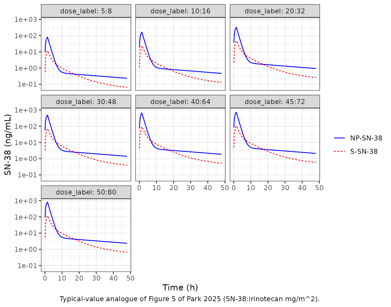
Visual predictive check of the totals (Figure 4)
A virtual cohort of 100 patients per dose level is simulated with between-subject variability on the trial sampling schedule (plus the end of the infusion, 1.5 h), and the median and 5th-95th percentiles of the predicted total irinotecan, total SN-38 and SN-38G are plotted (the source’s Figure 4 intervals also include residual error, so they are somewhat wider). Figure 1 of the source gives the observed medians by dose (for example, total SN-38 peaks above 100 ng/mL even at the lowest dose levels, and total irinotecan and SN-38 fall below 10 ng/mL within roughly a day).
rxode2::rxSetSeed(20251)
n_per <- 100
sample_times <- c(0, 0.5, 1, 1.5, 2, 4, 6, 8, 10, 12, 24, 36, 48, 72, 96, 120, 144, 169.5)
vpc_ev <- bind_rows(lapply(seq_len(nrow(cohorts)), function(i) {
  one <- snb101_events(cohorts$dose_sn38[i], cohorts$dose_iri[i], sample_times)
  bind_rows(lapply(seq_len(n_per), function(j) {
    mutate(one, id = (i - 1L) * n_per + j)
  }))
})) |>
  select(id, everything())

vpc <- as.data.frame(rxode2::rxSolve(mod, vpc_ev)) |>
  mutate(cohort = (as.integer(as.character(id)) - 1L) %/% n_per + 1L) |>
  left_join(cohorts |> select(cohort, dose_label), by = "cohort") |>
  transmute(
    id, time, dose_label,
    Irinotecan = Cc * mw[["irinotecan"]] / 1000,
    `SN-38` = Cc_sn38 * mw[["sn38"]] / 1000,
    `SN-38G` = Cc_sn38g * mw[["sn38g"]] / 1000
  )
#> ℹ parameter labels from comments will be replaced by 'label()'
vpc_sum <- vpc |>
  filter(time > 0) |>
  pivot_longer(c(Irinotecan, `SN-38`, `SN-38G`), names_to = "analyte", values_to = "conc") |>
  group_by(dose_label, analyte, time) |>
  summarise(
    p05 = quantile(conc, 0.05), p50 = median(conc), p95 = quantile(conc, 0.95),
    .groups = "drop"
  )
vpc_sum |>
  filter(time <= 72) |>
  ggplot(aes(time, p50)) +
  geom_ribbon(aes(ymin = p05, ymax = p95), fill = "steelblue", alpha = 0.25) +
  geom_line(colour = "red") +
  scale_y_log10() +
  facet_grid(analyte ~ dose_label, scales = "free_y") +
  labs(
    x = "Time (h)", y = "Total concentration (ng/mL)",
    caption = "Analogue of Figure 4 of Park 2025: simulated median (red) and 90% prediction interval."
  ) +
  theme_bw() +
  theme(axis.text.x = element_text(size = 7))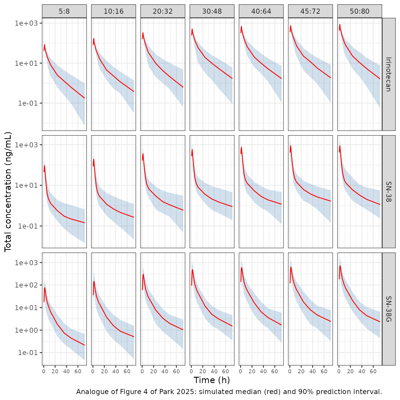
The simulated medians reproduce the shape and magnitude of the observed medians in Figure 1: at 50:80 mg/m^2, total irinotecan and total SN-38 both peak in the high hundreds of ng/mL at the end of the infusion, and SN-38G peaks a little later.
peak_50 <- vpc_sum |>
  filter(dose_label == "50:80") |>
  group_by(analyte) |>
  slice_max(p50, n = 1, with_ties = FALSE) |>
  ungroup()
knitr::kable(peak_50 |> select(analyte, time, p50) |>
rename(Analyte = analyte, `Time of peak median (h)` = time, `Peak median (ng/mL)` = p50), digits = 1)| Analyte | Time of peak median (h) | Peak median (ng/mL) |
|---|---|---|
| Irinotecan | 1.5 | 852.5 |
| SN-38 | 1.5 | 868.1 |
| SN-38G | 2.0 | 715.9 |
# Figure 1 at 50:80 mg/m^2: median total irinotecan peaks at about 800 ng/mL
# and total SN-38 at about 900 ng/mL. The bounds are deliberately wide (a
# factor of two); the structural check is the Table 3 replication above.
pk_med <- setNames(peak_50$p50, peak_50$analyte)
stopifnot(
  pk_med[["Irinotecan"]] > 400, pk_med[["Irinotecan"]] < 1600,
  pk_med[["SN-38"]] > 450, pk_med[["SN-38"]] < 1800
)
Assumptions and deviations
- Infusion duration, BSA and irinotecan molecular weight. None is stated in the paper. They were back-solved from Table 3 (see above): 1.6 m^2 from the AUCs, a 90-minute infusion from the NP-irinotecan Cmax, and the irinotecan hydrochloride molecular weight (623.1 g/mol) from the S-SN-38 AUC. The model file itself works in umol and does not depend on any of them; they matter only for converting mg/m^2 doses and for comparing with ng/mL values.
- Additive residual error. The supplementary control stream has a combined additive + proportional error for every analyte, with the additive term of total SN-38 fixed to 0.00001 and those of total irinotecan and SN-38G estimated (initial value 10 nmol/L). Table 2 reports only the three proportional terms, so the additive terms are omitted here and the model is proportional-only.
-
SN-38G peripheral compartment. Follows the
published control stream, in which the SN-38G peripheral compartment
does not return drug to the central compartment (see above), rather than
the reversible two-compartment exchange the text and Figure 2 describe.
peripheral1_sn38gis kept as a state so the model has the paper’s eleven compartments, but it does not affect any output. -
Fixed-to-zero etas omitted. The control stream
carries etas on Q1, k13, V8, V9, Q5, FMS and Q6, all fixed to 0; they
are left out.
FMS(the fraction of S-SN-38 clearance forming SN-38G) is fixed to 1 with no variability, so it is written into the micro-constants rather than carried as a parameter. - NP:S dose split in the event table. As in the source dataset, the 0.15:0.85 (irinotecan) and 0.98:0.02 (SN-38) composition is applied in the dosing records; the model has no bioavailability terms for it.
- Virtual cohort. Every simulated patient has BSA 1.6 m^2; the paper gives only cohort mean weights (68-75 kg), not BSA. The VPC uses 100 patients per dose level, not the trial cohort sizes, so that the percentiles are stable.
- Paper typo. The SN-38 NP/S Cmax ratio printed as 70.2% is 702% by the paper’s own per-mg/m^2 values.