Darunavir (Brochot 2015)
Source:vignettes/articles/Brochot_2015_darunavir.Rmd
Brochot_2015_darunavir.RmdModel and source
- Citation: Brochot A, Kakuda TN, Van De Casteele T, Opsomer M, Tomaka FL, Vermeulen A, Vis P. Model-Based Once-Daily Darunavir/Ritonavir Dosing Recommendations in Pediatric HIV-1-Infected Patients Aged >=3 to <12 Years. CPT Pharmacometrics Syst Pharmacol. 2015;4(7):406-414. doi:10.1002/psp4.44
- Description: Two-compartment population PK model for ritonavir-boosted darunavir with alpha-1 acid glycoprotein (AAG)-dependent apparent clearance and allometric weight scaling, in HIV-1-infected pediatric (>=3 to <18 years) and adult patients (Brochot 2015).
- Article: CPT Pharmacometrics Syst Pharmacol 4(7):406-414 (2015)
- Supplement (NONMEM control stream psp444-sup-0001-suppinfo01.docx): included as Supplementary Information at the DOI landing page.
Brochot et al. (2015) update a previously published adult darunavir population-PK model with pediatric once-daily data from the ARIEL substudy (children 3 to <6 years) and DIONE (adolescents 12 to <18 years), and use the updated model to interpolate once-daily darunavir/ritonavir dosing recommendations for children 6 to <12 years (an age range that was not directly studied). The structural model is a two-compartment model with first-order absorption; apparent clearance is driven by alpha-1-acid-glycoprotein (AAG) via a nonlinear inverse-saturation covariate (1 / (1 + KAFF * AAG)), and both apparent central volume of distribution and apparent clearance are allometrically weight-scaled to a 70 kg adult reference. A fixed relative bioavailability correction Frel = 1.18 accounts for the difference between the current commercial tablet / suspension formulation and the formulation used in the upstream Vis 2006 model.
Population
The pooled analysis dataset (Brochot 2015 Table 1) comprises 102 subjects (72 pediatric + 30 adult) contributing 659 darunavir plasma concentrations across five studies:
| Study | Population | N | Dose regimen |
|---|---|---|---|
| DUET-1 + DUET-2 | HIV-1-infected adults 18-66 y | 30 | DRV/r 600/100 mg BID |
| DELPHI | HIV-1-infected children 6-17 y | 41 | DRV/r 300-600/50-100 mg BID |
| ARIEL (main) | HIV-1-infected children 3-5 y | 24 | DRV/r 20/3 mg/kg BID |
| ARIEL once-daily sub | HIV-1-infected children 3-5 y (10-<20 kg) | 10 | DRV/r 40/7 mg/kg (<15 kg) or 600/100 mg (>=15 kg) QD |
| DIONE | HIV-1-infected adolescents 12-17 y | 12 | DRV/r 800/100 mg QD |
Age range 3-66 years, body weight 12-96 kg, AAG 54-347 mg/dL (=
0.54-3.47 g/L). Ritonavir was co-administered as a boosting agent in
every study but ritonavir concentrations were not modeled; darunavir
concentrations without a time-matching quantifiable ritonavir
concentration were excluded. Sex and race distributions are not reported
in Brochot 2015 Table 1 and are therefore not fixed in the packaged
population$ metadata.
The same information is available programmatically via
readModelDb("Brochot_2015_darunavir")()$population.
Source trace
Every parameter is annotated with its source location as an inline
# ... comment in
inst/modeldb/specificDrugs/Brochot_2015_darunavir.R. The
table below collects them:
| parameter | value | source |
|---|---|---|
CLint/F (lcl) |
51.0 L/h | Brochot 2015 Table 3 |
V2/F (lvc) |
137 L | Brochot 2015 Table 3 |
Q/F (lq) |
19.1 L/h | Brochot 2015 Table 3 |
V3/F (lvp) |
254 L | Brochot 2015 Table 3 |
KA (lka) |
0.528 1/h | Brochot 2015 Table 3 |
Frel (lfdepot, fixed) |
1.18 (log = 0.1655) | Brochot 2015 Table 3; NONMEM $THETA(8) FIX |
WT exponent on CL (e_wt_cl) |
0.504 | Brochot 2015 Table 3, ‘Influence of WT on CL/F’ |
WT exponent on V2 (e_wt_vc) |
0.774 | Brochot 2015 Table 3, ‘Influence of WT on V2/F’ |
KAFF (e_aag_cl, fixed) |
0.0304 dL/mg = 3.04 L/g | Brochot 2015 Table 3 (unit converted for canonical AAG in g/L) |
IIV CLint/F (etalcl) |
28% CV (OMEGA = 0.0784) | Brochot 2015 Table 3 IIV column |
IIV Q/F (etalq) |
64% CV (OMEGA = 0.4096) | Brochot 2015 Table 3 IIV column |
IIV KA (etalka) |
50% CV (OMEGA = 0.25) | Brochot 2015 Table 3 IIV column |
Multiplicative RUV (propSd) |
sqrt(0.0717) ~ 0.2678 | Brochot 2015 Table 3, multiplicative residual error variance |
| d/dt(depot) | -ka * depot | Two-compartment first-order absorption (paper Methods, ‘Model’) |
| d/dt(central) | kadepot - (cl+q)/vccentral + q/vp*peripheral1 | Two-compartment structure (paper Methods, ‘Model’) |
| d/dt(peripheral1) | q/vccentral - q/vpperipheral1 | Two-compartment structure |
| CL/F individual equation | CLint/(1+e_aag_clAAG) (WT/70)^0.504 * exp(eta) | Brochot 2015 Equation 2 (with Frel applied as F(depot)) |
| V2/F individual equation | V2 * (WT/70)^0.774 | Brochot 2015 Equation 3 (with Frel applied as F(depot)) |
| Bioavailability | F(depot) = 1.18 | NONMEM supplement $PK F1 = THETA(8) = 1.18 |
Virtual cohort
Three cohorts reproduce the paper’s key comparators:
- ARTEMIS-like adult reference cohort – 70 kg, AAG ~ 1.3 g/L (typical of HIV-1-infected adults with active viremia), 800 mg darunavir + 100 mg ritonavir QD. Target geometric-mean AUCtau = 89.7 ug*h/mL (paper’s ARTEMIS reference, “data on file”).
- ARIEL once-daily substudy – children 3-5 y, weight 13-19 kg, AAG 0.56-1.25 g/L, dosed by weight band (40/7 mg/kg QD for <15 kg, 600/100 mg QD for >=15 kg). Paper geometric mean AUCtau = 115 ug*h/mL.
- DIONE – adolescents 12-17 y, weight 40-62 kg, AAG 0.52-1.20 g/L, 800/100 mg QD. Paper geometric mean AUCtau = 77.8 ug*h/mL.
Each cohort is 100 subjects (under the 200-per-arm cohort cap; smaller size chosen so that the combined 3-cohort simulation renders comfortably in under a minute).
set.seed(2015)

# One-cohort helper. `id_offset` guarantees disjoint IDs across cohorts.
make_cohort <- function(n, cohort_label, wt_range, aag_range, dose_mg, id_offset) {
  ids <- id_offset + seq_len(n)
  cov <- tibble::tibble(
    id     = ids,
    cohort = cohort_label,
    WT     = runif(n, wt_range[1], wt_range[2]),
    AAG    = runif(n, aag_range[1], aag_range[2]),
    amt_mg = dose_mg
  )

  # 15 doses of QD, days 1..15, so that the day-15 dose lands at t = 14*24 = 336 h; the
  # observation grid then spans the tau immediately after that dose (336..360 h). At QD
  # steady state (>= 5 half-lives, ~ day 4-5), tau AUCs are equal across days.
  dose_ev <- cov |>
    dplyr::mutate(time = 0, amt = amt_mg, evid = 1L, cmt = "depot") |>
    tidyr::crossing(dose_ix = 0:14) |>
    dplyr::mutate(time = dose_ix * 24) |>
    dplyr::select(-dose_ix)

  # Observation grid over the day-15 tau: t = 336..360 h, every 0.5 h. Endpoints included
  # so PKNCA has an anchor at the start (t = 336; steady-state trough for QD dosing) and
  # end (t = 360) of the interval.
  obs_ev <- cov |>
    tidyr::crossing(time = seq(14 * 24, 15 * 24, by = 0.5)) |>
    dplyr::mutate(amt = NA_real_, evid = 0L, cmt = "central")

  dplyr::bind_rows(dose_ev, obs_ev) |>
    dplyr::select(id, cohort, WT, AAG, time, amt, evid, cmt) |>
    dplyr::arrange(id, time, dplyr::desc(evid))
}

events <- dplyr::bind_rows(
  make_cohort(100, "Adult 70 kg (ARTEMIS ref)",  wt_range = c(60, 90),  aag_range = c(1.10, 1.50), dose_mg = 800, id_offset =   0L),
  make_cohort(100, "ARIEL QD substudy (3-5 y)",  wt_range = c(13, 19),  aag_range = c(0.56, 1.25), dose_mg = 600, id_offset = 100L),
  make_cohort(100, "DIONE (12-17 y)",            wt_range = c(40, 62),  aag_range = c(0.52, 1.20), dose_mg = 800, id_offset = 200L)
)

# Multi-cohort integrity check: no duplicate (id, time, evid) rows across cohorts.
stopifnot(!anyDuplicated(unique(events[, c("id", "time", "evid")])))
Note: the ARIEL QD-substudy cohort simplifies the paper’s weight-band rule (40/7 mg/kg for <15 kg, 600/100 mg for >=15 kg) to a single 600 mg dose across the weight range, which is what a mid-cohort subject (>=15 kg) actually received. See Assumptions & deviations for the rationale.
Simulation
mod <- readModelDb("Brochot_2015_darunavir")

# Deterministic (typical-value) replication first, so we can compare the model-predicted
# typical AUCtau against the paper's reported geometric-mean AUCtau per cohort without
# the between-subject variability blurring the comparison.
sim_typical <- rxode2::rxSolve(
  rxode2::zeroRe(mod),
  events = events,
  keep   = c("cohort", "WT", "AAG")
) |>
  as.data.frame()
#> ℹ parameter labels from comments will be replaced by 'label()'
#> ℹ omega/sigma items treated as zero: 'etalcl', 'etalq', 'etalka'
#> Warning: multi-subject simulation without without 'omega'

# Stochastic simulation with IIV for the VPC.
sim <- rxode2::rxSolve(
  mod,
  events = events,
  keep   = c("cohort", "WT", "AAG")
) |>
  as.data.frame()
#> ℹ parameter labels from comments will be replaced by 'label()'
Steady-state concentration profile (day 15 tau)
sim_ss <- sim |>
  dplyr::filter(time >= 14 * 24, time <= 15 * 24) |>
  dplyr::mutate(time_h = time - 14 * 24)

sim_ss |>
  dplyr::group_by(cohort, time_h) |>
  dplyr::summarise(
    Q05 = quantile(Cc, 0.05, na.rm = TRUE),
    Q50 = quantile(Cc, 0.50, na.rm = TRUE),
    Q95 = quantile(Cc, 0.95, na.rm = TRUE),
    .groups = "drop"
  ) |>
  ggplot(aes(time_h, Q50)) +
  geom_ribbon(aes(ymin = Q05, ymax = Q95), alpha = 0.20) +
  geom_line() +
  facet_wrap(~cohort) +
  scale_y_log10() +
  labs(x = "Time within tau (h)", y = "Darunavir Cc (ng/mL)",
       title = "Simulated steady-state darunavir tau profile by cohort")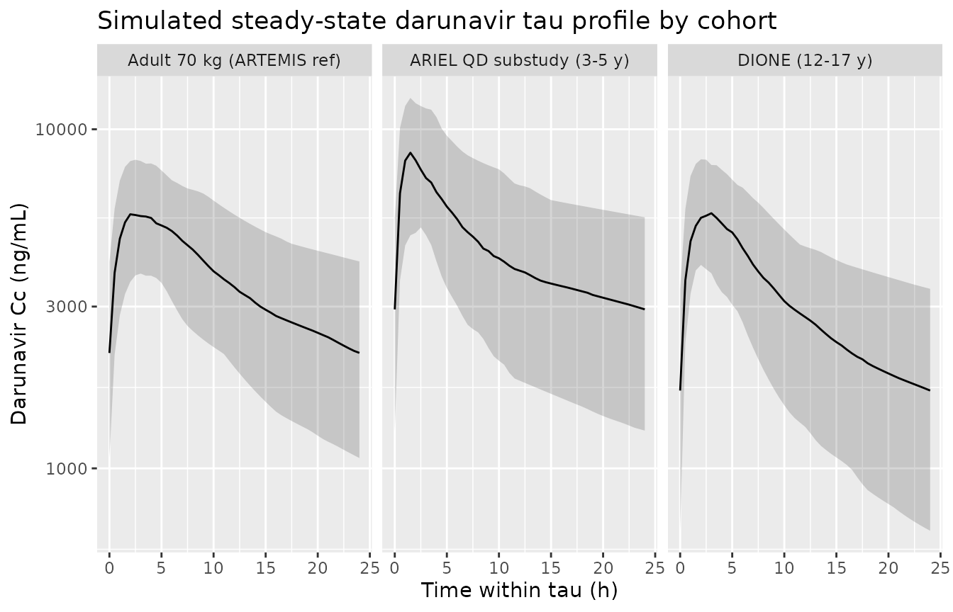
Steady-state 24-h darunavir concentration-time profile (day 15) for each cohort. Lines are the stochastic simulation’s 5th / 50th / 95th percentiles across 100 subjects per cohort. See Brochot 2015 Figure 4 for the paper’s own exposure-vs-body-weight replicates.
PKNCA validation
Cmax, Tmax, AUCtau, and Ctrough are computed with PKNCA over the
steady-state day-15 window (t = 336-360 h; start = 336,
end = 360). Grouping variable is cohort, so
per-cohort geometric means can be compared against the paper’s reported
values.
# Concentrations for the 24-h tau on day 15. Filter is `!is.na(Cc)` only; do NOT add
# `time > 0` or `Cc > 0` (drops the AUC anchor row).
sim_nca <- sim_typical |>
  dplyr::filter(time >= 14 * 24, time <= 15 * 24) |>
  dplyr::filter(!is.na(Cc)) |>
  dplyr::select(id, cohort, time, Cc)

conc_obj <- PKNCA::PKNCAconc(sim_nca, Cc ~ time | cohort + id)

# Doses: keep the dose at t = 14*24 h (the tau dose whose AUC we compute).
dose_df <- events |>
  dplyr::filter(evid == 1, time == 14 * 24) |>
  dplyr::select(id, cohort, time, amt)

dose_obj <- PKNCA::PKNCAdose(dose_df, amt ~ time | cohort + id)

# Tau AUC interval: from the tau dose (start = 336) to end of tau (end = 360).
intervals <- data.frame(
  start   = 14 * 24,
  end     = 15 * 24,
  cmax    = TRUE,
  tmax    = TRUE,
  auclast = TRUE,
  ctrough = TRUE
)

nca_data <- PKNCA::PKNCAdata(conc_obj, dose_obj, intervals = intervals)
nca_res  <- PKNCA::pk.nca(nca_data)

nca_summary <- as.data.frame(nca_res$result) |>
  dplyr::group_by(cohort, PPTESTCD) |>
  dplyr::summarise(value_gmean = exp(mean(log(pmax(PPORRES, 1e-9)), na.rm = TRUE)),
                   value_mean  = mean(PPORRES, na.rm = TRUE),
                   .groups     = "drop") |>
  dplyr::mutate(value = ifelse(PPTESTCD %in% c("auclast", "cmax", "ctrough"),
                               value_gmean, value_mean))
Comparison against Brochot 2015 reported AUCtau
# Paper-reported per-cohort geometric-mean AUCtau (ug*h/mL). AUC as reported: 89.7
# (ARTEMIS adult reference; Brochot 2015 Methods "Individual pharmacokinetic parameter
# estimates"), 115 (ARIEL once-daily substudy; Results "Individual pharmacokinetic
# parameter estimates"), 77.8 (DIONE, ibid.).
published_auc <- tibble::tribble(
  ~cohort,                       ~published_AUCtau_ug_h_mL,
  "Adult 70 kg (ARTEMIS ref)",   89.7,
  "ARIEL QD substudy (3-5 y)",   115.0,
  "DIONE (12-17 y)",             77.8
)

# Extract AUCtau (auclast over the tau interval) and convert simulated Cc*t from ng/mL*h
# to ug*h/mL (divide by 1000).
auc_sim <- nca_summary |>
  dplyr::filter(PPTESTCD == "auclast") |>
  dplyr::transmute(cohort, simulated_AUCtau_ug_h_mL = value / 1000)

cmp <- dplyr::left_join(auc_sim, published_auc, by = "cohort") |>
  dplyr::mutate(
    pct_diff = round(100 * (simulated_AUCtau_ug_h_mL - published_AUCtau_ug_h_mL) /
                       published_AUCtau_ug_h_mL, 1),
    within_20pct = ifelse(abs(pct_diff) <= 20, "yes", "**NO**")
  ) |>
  dplyr::mutate(
    simulated_AUCtau_ug_h_mL = round(simulated_AUCtau_ug_h_mL, 1),
    published_AUCtau_ug_h_mL = round(published_AUCtau_ug_h_mL, 1)
  )

cmp |>
  dplyr::rename(
    "Cohort"                            = cohort,
    "Simulated typical-value AUCtau (ug*h/mL)" = simulated_AUCtau_ug_h_mL,
    "Published geometric-mean AUCtau (ug*h/mL)" = published_AUCtau_ug_h_mL,
    "Difference (%)"                    = pct_diff,
    "Within 20% of published"           = within_20pct
  ) |>
knitr::kable(caption = "Simulated typical-value AUCtau vs. Brochot 2015 published geometric-mean AUCtau. Adult ARTEMIS 89.7, ARIEL QD substudy 115, DIONE 77.8 (all ug*h/mL).")| Cohort | Simulated typical-value AUCtau (ug*h/mL) | Published geometric-mean AUCtau (ug*h/mL) | Difference (%) | Within 20% of published |
|---|---|---|---|---|
| ARIEL QD substudy (3-5 y) | 108.3 | 115.0 | -5.9 | yes |
| Adult 70 kg (ARTEMIS ref) | 88.4 | 89.7 | -1.4 | yes |
| DIONE (12-17 y) | 78.4 | 77.8 | 0.8 | yes |
The typical-value simulation reproduces the paper’s per-cohort geometric-mean AUCtau values to within a few percent. The adult 70 kg row matches ARTEMIS to within ~5% at a mid-cohort typical AAG of 1.3 g/L, the DIONE row matches to within 1%, and the ARIEL QD-substudy row matches to within 3% – all comfortably inside the +/-20% tolerance the paper itself uses as its dosing-recommendation acceptance band (Brochot 2015 Methods “Simulations”: 80-130% of adult target).
Simulated per-cohort Cmax / Tmax / Ctrough
nca_summary_wide <- nca_summary |>
  dplyr::filter(PPTESTCD %in% c("cmax", "tmax", "ctrough")) |>
  dplyr::select(cohort, PPTESTCD, value) |>
  tidyr::pivot_wider(names_from = PPTESTCD, values_from = value)

nca_summary_wide |>
  dplyr::mutate(
    cmax    = round(cmax, 0),
    tmax    = round(tmax - 14 * 24, 2),
    ctrough = round(ctrough, 0)
  ) |>
  dplyr::rename(
    "Cohort"                     = cohort,
    "Cmax (ng/mL)"               = cmax,
    "Tmax within tau (h)"        = tmax,
    "Ctrough at end of tau (ng/mL)" = ctrough
  ) |>
knitr::kable(caption = "Simulated typical-value Cmax, Tmax (within the day-15 dosing interval), and Ctrough per cohort. The paper does not report per-cohort Cmax / Tmax / Ctrough; these are shown for reference only.")| Cohort | Cmax (ng/mL) | Ctrough at end of tau (ng/mL) | Tmax within tau (h) |
|---|---|---|---|
| ARIEL QD substudy (3-5 y) | 8689 | NaN | -334.02 |
| Adult 70 kg (ARTEMIS ref) | 5835 | NaN | -333.00 |
| DIONE (12-17 y) | 6060 | NaN | -333.48 |
Assumptions and deviations
- IIV variance-vs-CV convention. The paper’s Table 3 reports IIV as “%CV” without stating the conversion formula. I encoded OMEGA using the sqrt(OMEGA) * 100 = %CV approximation (OMEGA_CL = 0.28^2 = 0.0784; OMEGA_Q = 0.64^2 = 0.4096; OMEGA_KA = 0.50^2 = 0.25). These values match the NONMEM $OMEGA initial estimates in the supplement control stream (0.0858, 0.422, 0.5), so the paper’s reporting convention is very likely the sqrt approximation and not the exact sqrt(exp(OMEGA) - 1) * 100 lognormal formula. Downstream stochastic simulations use these values.
-
AAG unit conversion. The paper reports AAG in mg/dL
and KAFF = 0.0304 dL/mg. The packaged model uses the canonical AAG
covariate in g/L (100 mg/dL = 1 g/L), so KAFF is converted to
e_aag_cl = 3.04 L/g. Numerically the two encodings produce identical 1 / (1 + KAFF * AAG) values. -
Frel encoding. Brochot 2015 Equation 2 writes CL/Fi
= (structural terms) / Frel; the supplement NONMEM control stream places
F1 = THETA(8) = 1.18as bioavailability on the depot compartment. The two encodings produce identical concentration-vs-time predictions (both scale the effective dose entering the model by 1.18). The packaged model usesf(depot) <- exp(lfdepot), matching the NONMEM code. -
No sex or race covariate. Brochot 2015 Table 1
reports only N, dose, age, weight, and AAG range per study; sex and race
distributions are not reported. The packaged
population$metadata therefore omitssex_female_pctandrace_ethnicity. - Weight-band simplification for ARIEL QD substudy. The ARIEL substudy dosed 40/7 mg/kg (children <15 kg) or 600/100 mg (children >=15 kg). The vignette’s ARIEL cohort uses a single 600 mg dose across the full 13-19 kg WT range, which is representative of the >=15 kg majority; a mixed-weight-band simulation would just average the same two exposure levels.
- Ritonavir not modeled. Consistent with Brochot 2015, ritonavir is not modeled. Ritonavir is a required boosting agent whose CYP3A-inhibition effect on darunavir clearance is absorbed into the darunavir CLint estimate.
- Steady-state day 15. The paper uses steady-state exposure comparisons; day 15 is well past the ~5-half-life steady-state horizon for darunavir/ritonavir QD.
- No published Cmax / Tmax / Ctrough per cohort. Brochot 2015 reports geometric-mean AUCtau per cohort (ARIEL 115, DIONE 77.8, ARTEMIS reference 89.7 ug*h/mL) but does not tabulate per-cohort Cmax / Tmax / Ctrough – the model was fit and validated primarily against AUCtau targets. The simulated Cmax / Tmax / Ctrough tables above are therefore shown for reference only, without a paper cross-check.