Oxacillin (Murinova 2022)
Source:vignettes/articles/Murinova_2022_oxacillin.Rmd
Murinova_2022_oxacillin.RmdModel and source
#> ℹ parameter labels from comments will be replaced by 'label()'Citation: Murinova I, Svidrnoch M, Gucky T, Hlavac J, Michalek P, Slanar O, Sima M. Population Pharmacokinetic Analysis Proves Superiority of Continuous Infusion in PK/PD Target Attainment with Oxacillin in Staphylococcal Infections. Antibiotics (Basel). 2022;11(12):1736. doi:10.3390/antibiotics11121736
Description: One-compartment IV-infusion population PK model for oxacillin in 24 adult patients with staphylococcal infections, fitted to routine therapeutic-drug-monitoring total plasma concentrations (Murinova 2022). The model is parameterized by the volume of distribution (11.2 L, no covariate) and the elimination rate constant Ke, which carries an UNCENTERED exponential effect of the creatinine-based CKD-EPI eGFR expressed in mL/s/1.73 m2: Ke = 0.73 * exp(0.3 * eGFR) 1/h, i.e. 1.15 1/h (t1/2 0.6 h) at the cohort median eGFR of 1.53 mL/s/1.73 m2. Log-normal IIV on V and Ke; proportional residual error. An unbound concentration Cu = fu * Cc uses the cohort median measured protein binding of 86% (fu = 0.14), which the paper used to evaluate fT > MIC targets for intermittent, extended and continuous infusion.
This is a one-compartment intravenous oxacillin model fitted to
sparse routine therapeutic drug monitoring (TDM) data in adults treated
for staphylococcal infections. The authors parameterized it in the
volume of distribution (Vd) and the elimination rate
constant (Ke) rather than in clearance; the only retained
covariate is the CKD-EPI eGFR on Ke. The model’s purpose in
the paper is a Monte Carlo probability-of-target-attainment (PTA)
analysis on the unbound concentration, which showed
that the labelled intermittent 0.5-h infusions cannot hold unbound
oxacillin above the MIC for the whole dosing interval and that
continuous infusion can.
Population
24 adults (14 male, 10 female) treated with intravenous oxacillin for staphylococcal infection at the Military University Hospital in Prague between June 2021 and June 2022 contributed 32 total plasma concentrations (24 troughs and 8 post-infusion peaks; 1.33 per patient) (Murinova 2022 Results 2, Table 1, Methods 4.1). Median (IQR) age was 55 (45-72) years, body weight 84 (74-96) kg, BMI 28 (23-33) kg/m2 and serum albumin 32 (26-37) g/L. Renal function was preserved to moderately impaired: CKD-EPI eGFR 1.53 (0.98-1.71, range 0.59-2.10) mL/s/1.73 m2, i.e. about 92 (59-103, range 35-126) mL/min/1.73 m2. Patients on renal replacement therapy or extracorporeal life support were excluded. Infections were orthopedic (10), central nervous system (7), sepsis (3) and other (4); 21 were methicillin-susceptible Staphylococcus aureus, with a median MIC of 0.25 mg/L. Doses were 1-3 g every 4 h as 0.5-h infusions (one patient received 3-h extended infusions).
Unbound oxacillin was measured by ultrafiltration in the same samples; median plasma protein binding was 86% (IQR 83-88%, range 74-97%) and was not associated with any tested covariate, including albumin.
| Field | Value |
|---|---|
| species | human |
| n_subjects | 24 |
| n_studies | 1 |
| n_observations | 32 |
| age_range | 26-84 years |
| age_median | 55 years |
| weight_range | 57-145 kg |
| weight_median | 84 kg |
| sex_female_pct | 41.7 |
| disease_state | Staphylococcal infection treated with intravenous oxacillin: central nervous system (n = 7), orthopedic (n = 10), sepsis (n = 3), other (n = 4; e.g. bacteriuria, bacteremia, endocarditis). Methicillin-susceptible Staphylococcus aureus in 21 patients, S. hominis in 2, S. warneri in 1; MIC median 0.25 mg/L (IQR 0.25-0.5). |
| renal_function | eGFR (CKD-EPI, creatinine) median 1.53 mL/s/1.73 m2 (IQR 0.98-1.71, range 0.59-2.10), i.e. median 91.8 mL/min/1.73 m2 (range 35.4-126.0). Patients on renal replacement therapy or extracorporeal life support were excluded. |
| dose_range | 1-3 g every 4 h as a 0.5-h intravenous infusion; one patient received a 3-h extended infusion. |
| regions | Czech Republic (single centre: Military University Hospital Prague) |
| notes | Retrospective TDM study, June 2021 to June 2022 (Methods 4.1). 32 total plasma concentrations (24 troughs, 8 peaks after the end of infusion; 1.33 per patient). Total and ultrafiltrate-unbound oxacillin measured by LC-MS/MS; median protein binding 86% (IQR 83-88%, range 74-97%), not associated with any tested covariate. Estimation in Monolix 2021R1 (SAEM); Monte Carlo simulations in Simulx 2021. Demographics in Table 1. |
Source trace
Every value below is also carried as an in-file comment beside its
ini() entry in
inst/modeldb/specificDrugs/Murinova_2022_oxacillin.R.
| Equation / parameter | Value | Source location |
|---|---|---|
lvc (Vd) |
11.2 L | Table 2, Vd_pop (R.S.E. 30.4%) |
lkel (Ke at eGFR = 0) |
0.73 1/h | Table 2, Ke_pop (R.S.E. 26.1%) |
e_crcl_kel |
0.3 per mL/s/1.73 m2 | Table 2, beta_Ke_eGFR (R.S.E. 50.8%) |
etalvc |
0.7 SD -> 0.49 variance | Table 2, omega_Vd, under “Standard deviation of the
random effects” |
etalkel |
0.11 SD -> 0.0121 variance | Table 2, omega_Ke, same heading |
propSd |
0.4 | Table 2, error model parameter b; Results 2.1 “A
proportional error model” |
fu |
0.14 | Results 2, median protein binding 86% (IQR 83-88%) |
Log(Vd) = log(Vd_pop) + eta_Vd |
n/a | Results 2.1, first equation |
Log(Ke) = log(Ke_pop) + beta_Ke_eGFR x eGFR + eta_Ke |
n/a | Results 2.1, second equation |
d/dt(central) = -kel * central |
n/a | Results 2.1 “one-compartmental model with linear elimination kinetics” |
CRCL / 60 unit conversion |
n/a | Table 1 / Table 2 report eGFR in mL/s/1.73 m2; the canonical
CRCL column is mL/min/1.73 m2 |
Cu = fu * Cc |
n/a | Methods 4.6: PTA evaluated on “unbound oxacillin plasma concentration” |
The eGFR effect: printed equation versus prose
The paper describes the eGFR effect in two ways that do not agree
exactly. The Results 2.1 equation, which is Monolix’s standard covariate
form for a log-normally distributed parameter, is exponential:
Log(Ke) = log(Ke_pop) + beta x eGFR + eta_Ke, i.e.
Ke = 0.73 * exp(0.3 * eGFR). The abstract, Table 2 units
and the Discussion instead describe an additive effect, “Ke started at a
baseline of 0.73 h-1 and increased by 0.3 h-1 with each 1 mL/s/1.73 m2
of eGFR”, and the Discussion’s worked example (“In patients with an eGFR
of 1.5 mL/s/1.73 m2 … the oxacillin Ke was therefore 1.18 h-1, which
corresponds to the elimination half-life of 0.6 h”) uses that linear
reading: 0.73 + 0.3 * 1.5 = 1.18.
The model encodes the printed equation. Across the cohort’s eGFR range the two readings differ by at most about 4%, and both reproduce the reported half-life of 0.6 h:
egfr_si <- c(0.59, 0.98, 1.5, 1.53, 1.71, 2.10)
ke_forms <- tibble::tibble(
  eGFR_mL_s = egfr_si,
  Ke_equation = 0.73 * exp(0.3 * egfr_si),
  Ke_prose = 0.73 + 0.3 * egfr_si
) |>
  mutate(
    pct_diff = 100 * (Ke_equation / Ke_prose - 1),
    t_half_equation = log(2) / Ke_equation
  )
ke_forms |>
  mutate(across(-eGFR_mL_s, \(x) round(x, 3))) |>
  dplyr::rename(
    "eGFR (mL/s/1.73 m2)" = eGFR_mL_s,
    "Ke, printed equation (1/h)" = Ke_equation,
    "Ke, prose reading (1/h)" = Ke_prose,
    "% difference" = pct_diff,
    "t1/2, printed equation (h)" = t_half_equation
  ) |>
knitr::kable(caption = "Ke across Table 1's eGFR summary values under the two readings.")| eGFR (mL/s/1.73 m2) | Ke, printed equation (1/h) | Ke, prose reading (1/h) | % difference | t1/2, printed equation (h) |
|---|---|---|---|---|
| 0.59 | 0.871 | 0.907 | -3.930 | 0.795 |
| 0.98 | 0.980 | 1.024 | -4.345 | 0.708 |
| 1.50 | 1.145 | 1.180 | -2.977 | 0.605 |
| 1.53 | 1.155 | 1.189 | -2.841 | 0.600 |
| 1.71 | 1.219 | 1.243 | -1.905 | 0.568 |
| 2.10 | 1.371 | 1.360 | 0.784 | 0.506 |
# Deterministic algebra. The Discussion's t1/2 of 0.6 h at eGFR 1.5 holds
# under the encoded form (0.605 h); a wrong unit on eGFR (mL/min instead of
# mL/s) would give exp(0.3 * 90) and a t1/2 of essentially zero.
stopifnot(
  abs(ke_forms$t_half_equation[ke_forms$eGFR_mL_s == 1.5] - 0.6) < 0.05,
  all(abs(ke_forms$pct_diff) < 5)
)
The Monte Carlo replication of Table 3 below was run under both forms while the model was prepared; the exponential form matched the published PTAs as well as or slightly better than the linear one (for 1 g every 4 h, fT > MIC = 100% at MIC 0.25 mg/L, about 40% versus 35% against the published 41.5%), so nothing in the paper’s own simulations argues against the printed equation.
Typical-value solve against the closed form
mod <- readModelDb("Murinova_2022_oxacillin")

# Typical subject at the cohort median eGFR (1.53 mL/s/1.73 m2), one 1 g dose
# as a 0.5-h infusion.
typ_ev <- data.frame(
  id = 1L,
  time = c(0, seq(0.05, 8, by = 0.05)),
  evid = c(1L, rep(0L, 160)),
  amt = c(1000, rep(NA_real_, 160)),
  rate = c(2000, rep(NA_real_, 160)),
  cmt = "central",
  CRCL = 1.53 * 60
)
typ <- rxode2::rxSolve(
  rxode2::zeroRe(mod), events = typ_ev, rtol = 1e-10, atol = 1e-12
) |>
  as.data.frame()
#> ℹ parameter labels from comments will be replaced by 'label()'
#> ℹ omega/sigma items treated as zero: 'etalvc', 'etalkel'

k_typ <- 0.73 * exp(0.3 * 1.53)
v_typ <- 11.2
closed <- with(typ, ifelse(
  time <= 0.5,
  2000 / (k_typ * v_typ) * (1 - exp(-k_typ * time)),
  2000 / (k_typ * v_typ) * (1 - exp(-k_typ * 0.5)) * exp(-k_typ * (time - 0.5))
))
rel_err <- max(abs(typ$Cc / closed - 1))
rel_err
#> [1] 1.412616e-10
# Same parameters on both sides, so the difference is integrator error only
# (measured around 1e-9 at these tolerances).
stopifnot(rel_err < 1e-6, all(abs(typ$Cu / typ$Cc - 0.14) < 1e-12))
Virtual cohort
Individual data are not public. eGFR, the only retained covariate, is drawn by inverting a piecewise-linear interpolation of Table 1’s five-number summary (min 0.59, Q1 0.98, median 1.53, Q3 1.71, max 2.10 mL/s/1.73 m2). The quartiles are left-skewed (the median sits close to Q3), which a fitted log-normal cannot reproduce; quantile interpolation matches every published summary by construction.
# set.seed() fixes R's RNG (the covariate draw). rxode2's eta stream is
# partitioned per solver thread, so CI may draw different individuals; every
# Monte Carlo assertion below is on a cohort proportion or median with a bound
# at least 3 binomial standard errors wide.
set.seed(20221201)
rxode2::rxSetSeed(20221201)

n_arm <- 200L # cap is 200 per arm

sample_from_quantiles <- function(n, q) {
  stats::approx(
    x = c(0, 0.25, 0.5, 0.75, 1), y = q,
    xout = stats::runif(n), rule = 2
  )$y
}
draw_egfr <- function(n) sample_from_quantiles(n, c(0.59, 0.98, 1.53, 1.71, 2.10))

egfr_check <- stats::median(draw_egfr(n_arm))
egfr_check
#> [1] 1.569172
# A mis-entered quantile vector moves the median by tens of percent.
stopifnot(abs(egfr_check / 1.53 - 1) < 0.15)
# IV-infusion events as a plain data frame. Observation rows use the ODE state
# `central`, never the observable `Cc`; covariates are columns of this frame.
make_events <- function(regimen, dose_mg, tau_h, dur_h, n, id0, obs_grid,
                        end_h = 48) {
  ids <- id0 + seq_len(n)
  subj <- tibble::tibble(id = ids, eGFR = draw_egfr(n)) |>
    mutate(CRCL = eGFR * 60)
  doses <- subj |>
    tidyr::crossing(time = seq(0, end_h - tau_h, by = tau_h)) |>
    mutate(evid = 1L, amt = dose_mg, rate = dose_mg / dur_h)
  obs <- subj |>
    tidyr::crossing(time = obs_grid) |>
    mutate(evid = 0L, amt = NA_real_, rate = NA_real_)
  bind_rows(doses, obs) |>
    mutate(cmt = "central", regimen = regimen) |>
    arrange(id, time, desc(evid))
}
Simulation
Total concentrations under the observed regimen (Figure 2)
Figure 2 of the paper is a VPC of the total plasma concentrations. The study data are not available, so the figure below shows the model’s prediction interval (with residual error) for the most typical study regimen, 2 g every 4 h as a 0.5-h infusion, over the first day.
ev_obs <- make_events(
  "2 g q4h (0.5 h infusion)", 2000, 4, 0.5, n_arm, 0L,
  obs_grid = seq(0, 24, by = 0.1), end_h = 24
)
sim_obs <- rxode2::rxSolve(mod, events = ev_obs, keep = "regimen") |>
  as.data.frame()
#> ℹ parameter labels from comments will be replaced by 'label()'

sim_obs |>
  group_by(time) |>
  summarise(
    p10 = stats::quantile(sim, 0.10),
    p50 = stats::quantile(sim, 0.50),
    p90 = stats::quantile(sim, 0.90),
    .groups = "drop"
  ) |>
  ggplot(aes(time, p50)) +
  geom_ribbon(aes(ymin = pmax(p10, 0.01), ymax = p90), alpha = 0.25) +
  geom_line(linewidth = 0.7) +
  scale_y_log10() +
  scale_x_continuous(breaks = seq(0, 24, by = 4)) +
  labs(
    x = "Time (h)", y = "Total oxacillin (mg/L)",
    title = "2 g every 4 h, 0.5-h infusion",
    subtitle = "Median and 10th-90th percentiles including residual error, n = 200",
    caption = "Compare Figure 2 of Murinova 2022."
  )
#> Warning in scale_y_log10(): log-10 transformation introduced infinite values.
#> log-10 transformation introduced infinite values.
#> log-10 transformation introduced infinite values.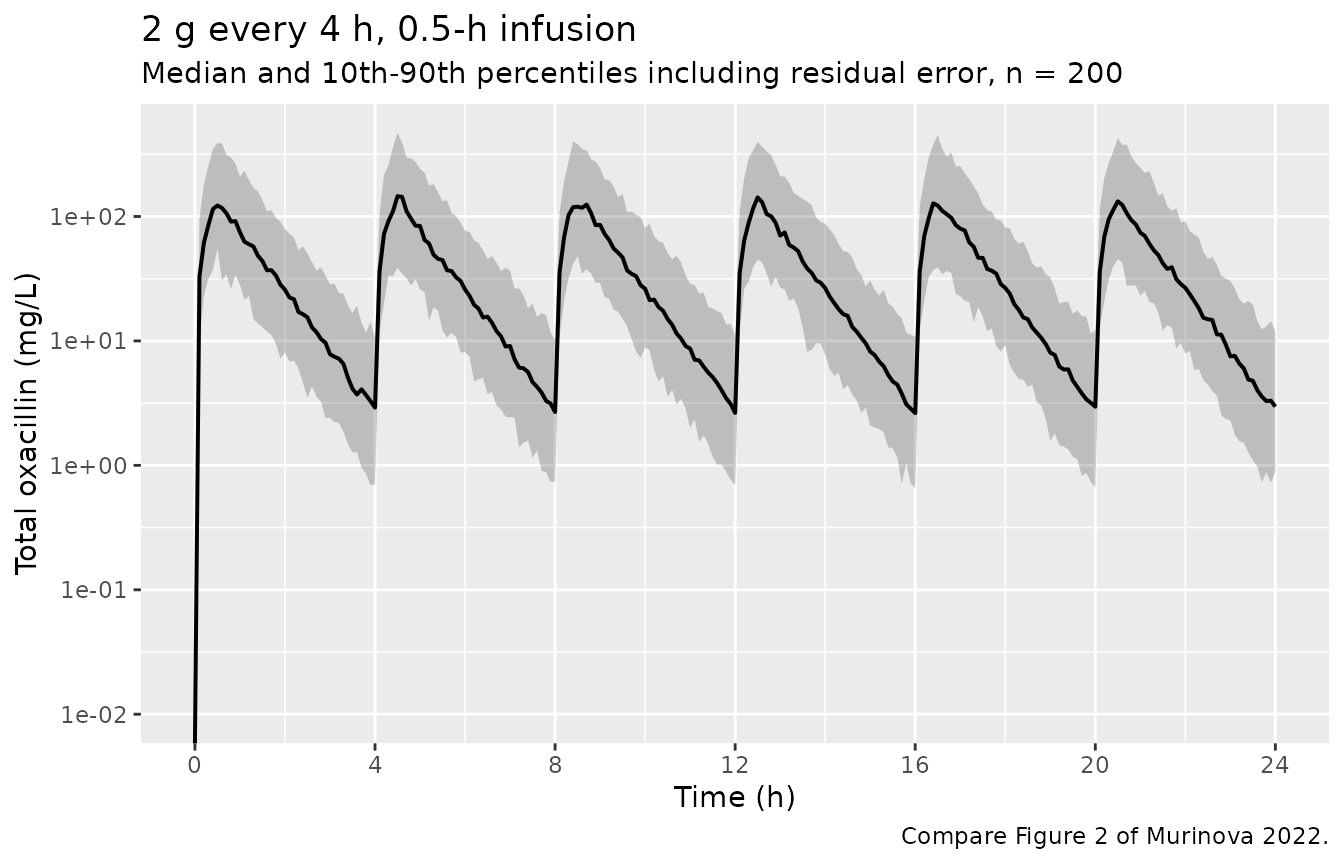
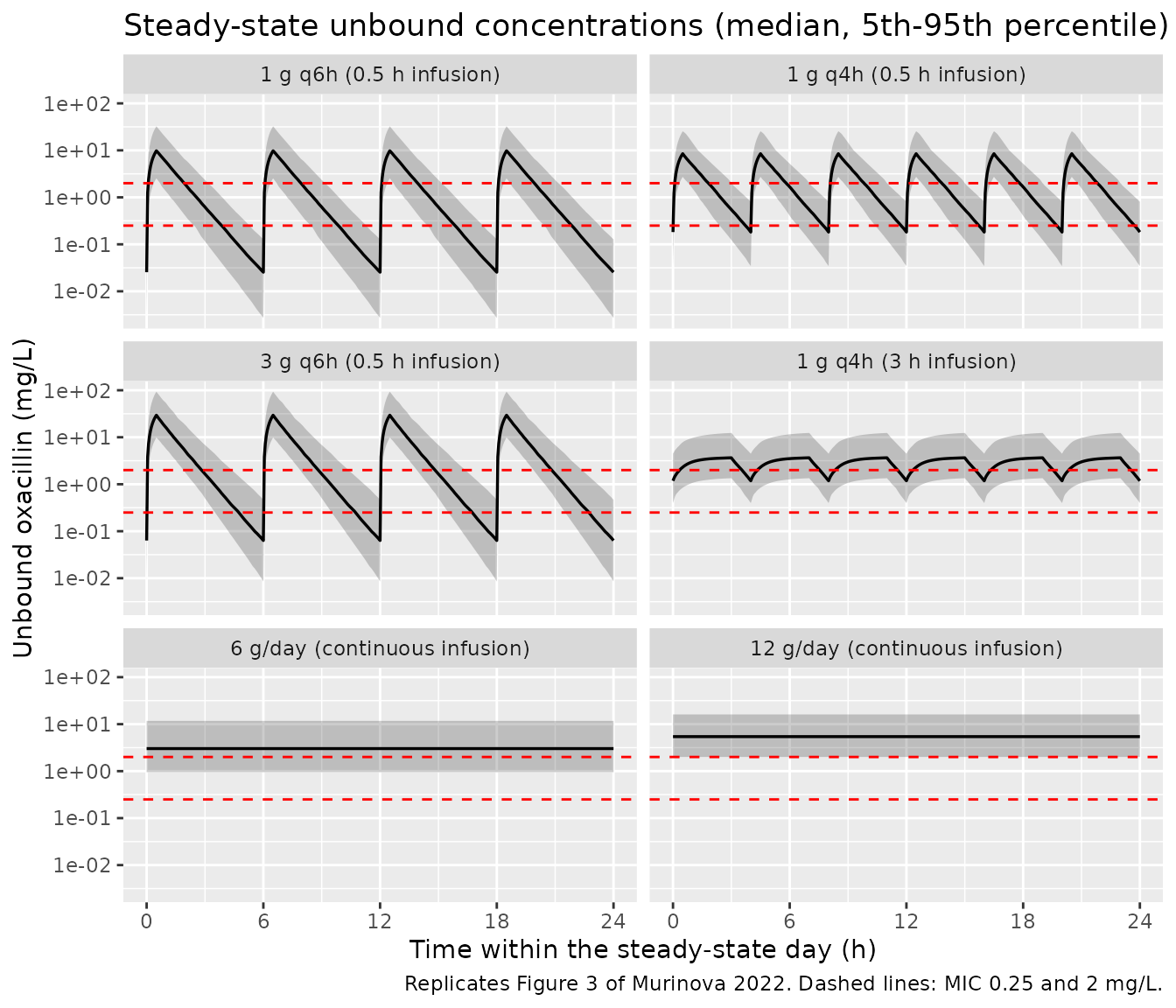
Unbound concentration profiles for the six simulated regimens (Figure 3)
regimens <- tibble::tribble(
  ~regimen,                         ~dose_mg, ~tau_h, ~dur_h,
  "1 g q6h (0.5 h infusion)",       1000,     6,      0.5,
  "1 g q4h (0.5 h infusion)",       1000,     4,      0.5,
  "3 g q6h (0.5 h infusion)",       3000,     6,      0.5,
  "1 g q4h (3 h infusion)",         1000,     4,      3,
  "6 g/day (continuous infusion)",  6000,     24,     24,
  "12 g/day (continuous infusion)", 12000,    24,     24
)

# Steady state is reached well within the first 24 h (t1/2 at most about
# 1.1 h at the lowest Ke in the cohort), so the PTA window is 24-48 h.
pta_grid <- seq(24, 48, by = 0.05)
ev_reg <- bind_rows(lapply(seq_len(nrow(regimens)), function(i) {
  make_events(
    regimens$regimen[i], regimens$dose_mg[i], regimens$tau_h[i],
    regimens$dur_h[i], n_arm, (i - 1L) * n_arm, obs_grid = pta_grid
  )
}))
sim_reg <- rxode2::rxSolve(mod, events = ev_reg, keep = "regimen") |>
  as.data.frame() |>
  mutate(regimen = factor(regimen, levels = regimens$regimen))
stopifnot(!anyNA(sim_reg$Cu))
sim_reg |>
  group_by(regimen, time) |>
  summarise(
    p05 = stats::quantile(Cu, 0.05),
    p50 = stats::quantile(Cu, 0.50),
    p95 = stats::quantile(Cu, 0.95),
    .groups = "drop"
  ) |>
  ggplot(aes(time - 24, p50)) +
  geom_ribbon(aes(ymin = p05, ymax = p95), alpha = 0.25) +
  geom_line(linewidth = 0.6) +
  geom_hline(yintercept = c(0.25, 2), colour = "red", linetype = "dashed") +
  facet_wrap(~regimen, ncol = 2) +
  scale_y_log10() +
  scale_x_continuous(breaks = seq(0, 24, by = 6)) +
  labs(
    x = "Time within the steady-state day (h)", y = "Unbound oxacillin (mg/L)",
    title = "Steady-state unbound concentrations (median, 5th-95th percentile)",
    caption = "Replicates Figure 3 of Murinova 2022. Dashed lines: MIC 0.25 and 2 mg/L."
  )
Replicating Table 3 – probability of target attainment
A subject attains the target when its unbound concentration stays above the MIC for 100% (or at least 50%) of the steady-state day. The paper simulated 500 replicates of its 24 patients in Simulx; here each regimen uses 200 virtual patients, so each PTA carries a binomial standard error of up to 3.5 percentage points.
pta_sub <- sim_reg |>
  filter(time < 48) |>
  group_by(regimen, id) |>
  summarise(
    ft_025 = mean(Cu > 0.25),
    ft_2 = mean(Cu > 2),
    .groups = "drop"
  )
pta_sim <- pta_sub |>
  group_by(regimen) |>
  summarise(
    sim_100_025 = 100 * mean(ft_025 >= 1),
    sim_100_2 = 100 * mean(ft_2 >= 1),
    sim_50_025 = 100 * mean(ft_025 >= 0.5),
    sim_50_2 = 100 * mean(ft_2 >= 0.5),
    .groups = "drop"
  )

pta_paper <- tibble::tibble(
  regimen = factor(regimens$regimen, levels = regimens$regimen),
  pub_100_025 = c(4.35, 41.52, 17.56, 95.30, 99.82, 99.97),
  pub_100_2 = c(0.05, 2.60, 0.64, 32.23, 69.95, 90.72),
  pub_50_025 = c(60.83, 60.25, 87.77, 99.93, 99.82, 99.97),
  pub_50_2 = c(5.55, 27.69, 27.48, 72.40, 69.95, 90.72)
)
pta_cmp <- left_join(pta_paper, pta_sim, by = "regimen")

pta_cmp |>
  mutate(across(where(is.numeric), \(x) round(x, 1))) |>
  dplyr::select(
    regimen, pub_100_025, sim_100_025, pub_100_2, sim_100_2,
    pub_50_025, sim_50_025, pub_50_2, sim_50_2
  ) |>
  dplyr::rename(
    "Regimen" = regimen,
    "100%, 0.25: published" = pub_100_025,
    "100%, 0.25: simulated" = sim_100_025,
    "100%, 2: published" = pub_100_2,
    "100%, 2: simulated" = sim_100_2,
    "50%, 0.25: published" = pub_50_025,
    "50%, 0.25: simulated" = sim_50_025,
    "50%, 2: published" = pub_50_2,
    "50%, 2: simulated" = sim_50_2
  ) |>
  knitr::kable(caption = paste(
    "PTA (%) by fT > MIC target (100% or 50%) and MIC (mg/L).",
    "Published values from Table 3 of Murinova 2022."
))| Regimen | 100%, 0.25: published | 100%, 0.25: simulated | 100%, 2: published | 100%, 2: simulated | 50%, 0.25: published | 50%, 0.25: simulated | 50%, 2: published | 50%, 2: simulated |
|---|---|---|---|---|---|---|---|---|
| 1 g q6h (0.5 h infusion) | 4.3 | 1.5 | 0.0 | 0 | 60.8 | 87 | 5.6 | 8.5 |
| 1 g q4h (0.5 h infusion) | 41.5 | 38.5 | 2.6 | 1 | 60.2 | 100 | 27.7 | 36.5 |
| 3 g q6h (0.5 h infusion) | 17.6 | 13.0 | 0.6 | 0 | 87.8 | 99 | 27.5 | 43.5 |
| 1 g q4h (3 h infusion) | 95.3 | 98.5 | 32.2 | 23 | 99.9 | 100 | 72.4 | 71.5 |
| 6 g/day (continuous infusion) | 99.8 | 100.0 | 70.0 | 74 | 99.8 | 100 | 70.0 | 74.0 |
| 12 g/day (continuous infusion) | 100.0 | 100.0 | 90.7 | 95 | 100.0 | 100 | 90.7 | 95.0 |
The headline conclusions reproduce: no 0.5-h infusion regimen reaches 90% PTA for the optimal target, the 3-h extended infusion does so only at MIC 0.25 mg/L, and at MIC 2 mg/L only 12 g/day by continuous infusion clears 90%. The fT > MIC = 100% columns and the continuous-infusion rows match closely.
The fT > MIC = 50% column for the 0.5-h infusion regimens does not reproduce. The published values are internally inconsistent with a steady-state PK simulation: Table 3 reports a lower PTA for 1 g every 4 h (60.25%) than for 1 g every 6 h (60.83%) at MIC 0.25 mg/L, although the 4-h regimen delivers 50% more drug and spends a larger fraction of every interval above any given MIC. That ordering is impossible for any single set of individual parameters, so the 50% column was probably derived differently (for example over a non-steady-state window) in Simulx. These cells are shown but not asserted.
row <- function(r) pta_cmp[pta_cmp$regimen == r, ]
ci12 <- row("12 g/day (continuous infusion)")
ci6 <- row("6 g/day (continuous infusion)")
ext <- row("1 g q4h (3 h infusion)")
std6 <- row("1 g q6h (0.5 h infusion)")

# Model-true values (from 24 x 500 closed-form replicates while preparing the
# model): CI 12 g MIC 2 ~ 92%, CI 6 g MIC 2 ~ 69%, extended MIC 0.25 ~ 98%,
# standard q6h MIC 0.25 ~ 2%. With n = 200 the binomial SE is at most 3.3
# points, so 12- and 15-point bounds sit more than 3 SE from each estimate,
# while a wrong eGFR unit, a variance/SD mix-up on Vd (0.7 vs 0.49), or a
# missing fu moves these by tens of points.
stopifnot(
  abs(ci12$sim_100_2 - ci12$pub_100_2) < 12,
  abs(ci6$sim_100_2 - ci6$pub_100_2) < 15,
  ext$sim_100_025 > 85,
  std6$sim_100_025 < 15,
  ci12$sim_100_2 > ci6$sim_100_2
)
eGFR-graded continuous infusion
The paper’s dosing proposal gives 9.5 g/day by continuous infusion for eGFR 0.5-1.0, 11 g/day for 1.0-1.5 and 12.5 g/day above 1.5 mL/s/1.73 m2, and reports a pooled PTA of 90.18% for fT > MIC = 100% at MIC 2 mg/L.
ev_graded <- make_events(
  "graded", 1, 24, 24, n_arm, 10000L, obs_grid = seq(24, 48, by = 0.5)
) |>
  mutate(
    daily_mg = case_when(eGFR <= 1.0 ~ 9500, eGFR <= 1.5 ~ 11000, TRUE ~ 12500),
    amt = ifelse(evid == 1L, daily_mg, NA_real_),
    rate = ifelse(evid == 1L, daily_mg / 24, NA_real_)
  )
sim_graded <- rxode2::rxSolve(mod, events = ev_graded, keep = "daily_mg") |>
  as.data.frame()

pta_graded <- sim_graded |>
  filter(time < 48) |>
  group_by(id, daily_mg) |>
  summarise(ok = all(Cu > 2), .groups = "drop")
pta_graded_pct <- 100 * mean(pta_graded$ok)
c(simulated = pta_graded_pct, published = 90.18)
#> simulated published
#>     92.50     90.18
# Model-true ~ 90%; SE ~ 2.1 points at n = 200.
stopifnot(abs(pta_graded_pct - 90.18) < 10)
PKNCA validation
A single 1 g dose as a 0.5-h infusion in the 200-subject cohort. The paper reports no NCA; its only reported exposure summary is the Discussion’s elimination half-life of 0.6 h at eGFR 1.5 mL/s/1.73 m2, which is the reference below (the cohort median eGFR is 1.53).
ev_sd <- make_events(
  "1 g single dose (0.5 h infusion)", 1000, 24, 0.5, n_arm, 20000L,
  obs_grid = c(0, 0.25, 0.5, 0.75, 1, 1.5, 2, 3, 4, 5, 6, 8), end_h = 24
)
sim_sd <- rxode2::rxSolve(
  rxode2::zeroRe(mod, "sigma"), events = ev_sd, keep = "regimen"
) |>
  as.data.frame() |>
  dplyr::rename(treatment = regimen)
#> ℹ parameter labels from comments will be replaced by 'label()'

# Integrator undershoot near zero is noise; floor it, and keep the time-zero
# row so AUC is anchored at 0.
stopifnot(all(sim_sd$Cc >= -1e-6 * max(sim_sd$Cc)))
conc_sd <- sim_sd |>
  dplyr::filter(!is.na(Cc)) |>
  mutate(Cc = pmax(Cc, 0)) |>
  select(id, time, Cc, treatment)
dose_sd <- ev_sd |>
  filter(evid == 1L) |>
  select(id, time, amt, treatment = regimen)

nca_res <- PKNCA::pk.nca(PKNCA::PKNCAdata(
  PKNCA::PKNCAconc(conc_sd, Cc ~ time | treatment + id),
  PKNCA::PKNCAdose(dose_sd, amt ~ time | treatment + id),
  intervals = data.frame(
    start = 0, end = Inf,
    cmax = TRUE, tmax = TRUE, aucinf.obs = TRUE, half.life = TRUE
  )
))

nca_ref <- data.frame(
  treatment = "1 g single dose (0.5 h infusion)",
  half.life = 0.6
)
nca_tbl <- nlmixr2lib::ncaComparisonTable(
  nca_res, nca_ref,
  by = "treatment",
  params = "half.life",
  units = c(half.life = "h")
)
knitr::kable(nca_tbl, caption = "Median simulated NCA half-life vs. the Discussion's 0.6 h.")| NCA parameter | treatment | Reference | Simulated | % diff |
|---|---|---|---|---|
| t½ (h) | 1 g single dose (0.5 h infusion) | 0.6 | 0.633 | +5.5% |
nca_df <- as.data.frame(nca_res)
med_hl <- stats::median(nca_df$PPORRES[nca_df$PPTESTCD == "half.life"])
med_auc <- stats::median(nca_df$PPORRES[nca_df$PPTESTCD == "aucinf.obs"])
c(median_half_life_h = med_hl, median_aucinf_mg_h_L = med_auc)
#>   median_half_life_h median_aucinf_mg_h_L
#>            0.6328649           88.7206785
# Median half-life: model-true about log(2) / (0.73 * exp(0.3 * 1.53)) = 0.60 h
# with only 11% IIV on Ke; robust to the draw.
stopifnot(abs(med_hl / 0.6 - 1) < 0.15)
nca_df |>
  filter(PPTESTCD %in% c("cmax", "tmax", "aucinf.obs", "half.life")) |>
  group_by(PPTESTCD) |>
  summarise(
    median = stats::median(PPORRES),
    p05 = stats::quantile(PPORRES, 0.05),
    p95 = stats::quantile(PPORRES, 0.95),
    .groups = "drop"
  ) |>
  mutate(across(where(is.numeric), \(x) signif(x, 3))) |>
  dplyr::rename(
    "NCA parameter" = PPTESTCD,
    "Median" = median,
    "5th percentile" = p05,
    "95th percentile" = p95
  ) |>
knitr::kable(caption = "Single-dose NCA across the virtual cohort (1 g, 0.5-h infusion).")| NCA parameter | Median | 5th percentile | 95th percentile |
|---|---|---|---|
| aucinf.obs | 88.700 | 23.800 | 234.000 |
| cmax | 74.100 | 19.900 | 189.000 |
| half.life | 0.633 | 0.484 | 0.824 |
| tmax | 0.500 | 0.500 | 0.500 |
Assumptions and deviations
-
eGFR effect form. The printed Results 2.1 equation
(
Log(Ke) = log(Ke_pop) + beta x eGFR + eta, exponential) is encoded. The prose, Table 2 units and the Discussion’s worked example (Ke 1.18 1/h at eGFR 1.5) read the same coefficient as an additive 0.3 1/h per mL/s/1.73 m2. Within the cohort’s eGFR range the two readings differ by under 5%; see The eGFR effect above. -
eGFR units. The paper reports eGFR in mL/s/1.73 m2;
the model takes the canonical
CRCLin mL/min/1.73 m2 and divides by 60. The effect is uncentered, solkelis Ke at eGFR = 0, not a typical value. - Random effects. Table 2 reports the random effects as standard deviations (0.7 on Vd, 0.11 on Ke); they are squared to variances. The 0.7 SD on Vd is large (CV about 80%) and reflects sparse, trough-dominated sampling (24 of 32 samples were troughs).
-
Unbound fraction.
fu = 0.14is the cohort median of the measured protein binding (86%) and is fixed for every subject. The paper does not state how unbound concentrations were generated in Simulx; a fixed median fraction is the simplest reading and reproduces the continuous-infusion PTAs. Measured binding ranged from 74% to 97%, so an individual’s unbound exposure can differ fromCuby roughly a factor of two either way. - Covariate distribution. eGFR is drawn from Table 1’s five-number summary by quantile interpolation; the individual values are not published.
- PTA definition. fT > MIC is evaluated on the unbound concentration without residual error over the second (steady-state) day. The fT > MIC = 50% column for the 0.5-h infusion regimens of Table 3 does not reproduce and appears internally inconsistent (see above).
- Errata. No erratum or correction for this article was found (checked 2026-10-10).