Factor IX (Brekkan 2016)

Model and source

• Citation: Brekkan A, Berntorp E, Jensen K, Nielsen EI, Jonsson S. Population pharmacokinetics of plasma-derived factor IX: procedures for dose individualization. J Thromb Haemost. 2016;14(4):724-732. doi:[10.1111/jth.13271](https://doi.org/10.1111/jth.13271)
• Description: Three-compartment population PK model for plasma-derived factor IX (FIX) activity in patients with moderate or severe haemophilia B.
• Article: https://doi.org/10.1111/jth.13271
• Modality: Plasma-derived FIX concentrate, IV infusion.

Brekkan 2016 reevaluated a previously published three-compartment popPK model for plasma-derived FIX activity (the “original model” of Berntorp et al., reference 15 in the paper) using an extended pooled data set, and used the refit to explore sparse sampling schedules for individual Bayesian dose prediction in haemophilia B. The packaged model implements the final re-estimated model (Brekkan 2016 Table 2, with equations in Material and methods, p. 725): three-compartment disposition with IV input and first-order elimination from the central compartment, allometric weight scaling on all CL / Q (exponent 0.75) and V (exponent 1.0) parameters with reference weight 70 kg, an endogenous FIX-activity baseline estimated as a structural parameter, two correlated IIV blocks (CL/V1 and V2/V3) plus an independent IIV on baseline, and a combined additive + proportional residual error. The final model has five fewer parameters than the original Berntorp model and an OFV 1941 points lower (Brekkan 2016 Results, p. 727).

Population

The development cohort comprised 34 unique patients with moderate or severe haemophilia B pooled across five previously published studies (Brekkan 2016 Table 1):

• 1,794 FIX activity samples; 7-17 samples per patient per occasion; 35 samples below the typical 0.01 U/mL limit of quantification were retained in the data set.
• Mean body weight 66.8 (SD 13.5) kg; per-study means 61.0-69.7 kg.
• Mean age 27.5 (SD 10.9) years; per-study means 23.1-42.8 years.
• Sex: haemophilia B is X-linked recessive, so the cohort is essentially all male.
• Race / ethnicity: not reported.
• Disease state: moderate or severe haemophilia B; baseline FIX activity estimated as a model parameter (0.01588 U/mL typical value).
• Products: seven plasma-derived FIX concentrates (AlphaNine - the most common - plus Factor IX Grifols, Immunine, Octanine, Nanotiv, Preconativ, Mononine). Product was tested as a covariate on CL and dropped from the final model because no product changed typical CL by more than 20% (Brekkan 2016 Results, p. 727).
• Sampling can in general be considered single-dose PK; the shortest and longest time periods between occasions were 4 days and > 4 years.

The Discussion notes the final model should be used with caution to describe FIX activity following administration of products that are not plasma-derived. The same metadata is available programmatically via readModelDb("Brekkan_2016_factorIX")$population.

Source trace

The per-parameter origin is recorded as an in-file comment next to each ini() entry in inst/modeldb/specificDrugs/Brekkan_2016_factorIX.R. The table below collects them in one place for review.

Parameter (model name)	Value	Source
lcl (typical CL, mL/h)	log(319.8)	Brekkan 2016 Table 2: CL = 319.8 mL/h
lvc (typical V1, mL)	log(5922)	Brekkan 2016 Table 2: V1 = 5922 mL
lvp (typical V2, mL)	log(828.9)	Brekkan 2016 Table 2: V2 = 828.9 mL
lq (typical Q2, mL/h)	log(1049)	Brekkan 2016 Table 2: Q2 = 1049 mL/h
lvp2 (typical V3, mL)	log(2234)	Brekkan 2016 Table 2: V3 = 2234 mL
lq2 (typical Q3, mL/h)	log(160.4)	Brekkan 2016 Table 2: Q3 = 160.4 mL/h
lrbase (endogenous baseline, U/mL)	log(0.01588)	Brekkan 2016 Table 2: baseline FIX activity = 0.01588 U/mL
Allometric exponent on CL, Q2, Q3	0.75 (fixed)	Brekkan 2016 Methods p. 725 and Results p. 727 (three approaches gave similar fits)
Allometric exponent on V1, V2, V3	1.00 (fixed)	Brekkan 2016 Methods p. 725: volume exponent fixed at 1
Reference body weight	70 kg	Brekkan 2016 Table 2 footnote (typical value defined for 70 kg subject)
IIV block etalcl + etalvc	c(0.016129, 0.014053, 0.024649)	Brekkan 2016 Table 2: x_CL = 0.127, x_V1 = 0.157, corr(CL,V1) = 0.705
IIV block etalvp + etalvp2	c(0.444889, 0.553828, 1.040400)	Brekkan 2016 Table 2: x_V2 = 0.667, x_V3 = 1.020, corr(V2,V3) = 0.814
etalrbase (IIV on baseline)	0.042849	Brekkan 2016 Table 2: x_BASELINE = 0.207
propSd (proportional residual)	0.0695	Brekkan 2016 Table 2: proportional residual error = 0.0695
addSd (additive residual, U/mL)	0.0067	Brekkan 2016 Table 2: additive residual error = 0.0067 U/mL
Equation: d/dt(central)	n/a	Brekkan 2016 Material and methods, p. 725 (three-compartment IV model)
Equation: d/dt(peripheral1)	n/a	Brekkan 2016 Material and methods, p. 725
Equation: d/dt(peripheral2)	n/a	Brekkan 2016 Material and methods, p. 725
Equation: Cc = central / vc + rbase	n/a	Brekkan 2016 Material and methods, p. 725 (baseline estimated as structural parameter)

The IIV values are reported in Table 2 under the heading “coefficient of variation of interindividual variability of clearance, volumes and baseline”. The Brekkan 2016 paper does not include a sqrt(variance) * 100 footnote directly, but the sister factor IX papers from the same modelling lineage do (Diao 2014 Table 3 footnote: “IIV calculated as sqrt(variance) * 100”; Koopman 2023 Table 2 footnote: “IIV and IOV coefficient of variation calculated as: sqrt(variance) * 100%”). Under that convention the reported value equals the SD of the log-scale eta directly, so omega^2 = (reported_value)^2 and cov = corr * sqrt(var1) * sqrt(var2). This is the convention encoded in the packaged model file. See Assumptions and deviations for the small-IIV check.

The final model also estimated inter-occasion variability on CL (21.4% CV) and V1 (20.1% CV) with correlation 0.902 between the two random effects (Brekkan 2016 Table 2). IOV is not implemented in this static library model because the library event grid has no occasion variable; see Assumptions and deviations.

Virtual cohort

Original observed FIX activity data are not publicly available. The simulations below use a virtual cohort whose demographics approximate the Brekkan 2016 development population: body weight is sampled around the cohort mean of 66.8 kg (capped to a plausible adult haemophilia B range). Per Brekkan 2016 simulation design (p. 726) all simulated patients are assigned a baseline FIX activity of 0 U/mL to represent severe haemophilia B; this is implemented in the rxode2 call by overriding rbase = 0.

set.seed(2016)

n_per_group <- 100L

cohort <- tibble(
  ID        = seq_len(n_per_group),
  WT        = pmin(pmax(rlnorm(n_per_group, log(66.8), 0.18), 45), 110),
  treatment = "39 U/kg Mon+Thu"
)

stopifnot(!anyDuplicated(cohort$ID))
summary(cohort)
#>        ID               WT            treatment  
#>  Min.   :  1.00   Min.   :45.00   Length   :100  
#>  1st Qu.: 25.75   1st Qu.:58.71   N.unique :  1  
#>  Median : 50.50   Median :63.67   N.blank  :  0  
#>  Mean   : 50.50   Mean   :66.54   Min.nchar: 15  
#>  3rd Qu.: 75.25   3rd Qu.:74.31   Max.nchar: 15  
#>  Max.   :100.00   Max.   :99.15

The simulation replicates Brekkan 2016 Figure 1: eight 10-min IV infusions of 39 U/kg administered on Mondays and Thursdays (interval 72 h, then 96 h, alternating), with dense sampling after the eighth dose for 96 h. The 8th (final) dose is on the second Thursday of the third week (study day 24).

infusion_min <- 10
infusion_h   <- infusion_min / 60

# Dose times in hours (relative to t = 0 on Monday of week 1):
# Mon week1 = 0; Thu week1 = 72; Mon week2 = 168; Thu week2 = 240;
# Mon week3 = 336; Thu week3 = 408; Mon week4 = 504; Thu week4 = 576.
dose_times <- c(0, 72, 168, 240, 336, 408, 504, 576)
last_dose  <- max(dose_times)

# 22-point sampling schedule (Brekkan 2016 Fig. 1) after the last dose,
# expressed as hours after t = 0:
post_last  <- c(0, 0.1, 0.5, 1, 2, 4, 6, 12, 18, 24, 30, 36,
                42, 48, 54, 60, 66, 72, 78, 84, 90, 96)
obs_times  <- last_dose + post_last

build_events <- function(pop) {
  dose <- pop |>
    tidyr::crossing(start = dose_times) |>
    mutate(
      AMT  = WT * 39,
      RATE = AMT / infusion_h,
      TIME = start,
      EVID = 1,
      CMT  = "central",
      DV   = NA_real_
    ) |>
    select(-start)
  obs <- pop |>
    tidyr::crossing(TIME = obs_times) |>
    mutate(AMT = NA_real_, RATE = NA_real_,
           EVID = 0, CMT = "central", DV = NA_real_)
  bind_rows(dose, obs) |>
    arrange(ID, TIME, desc(EVID)) |>
    as.data.frame()
}

events <- build_events(cohort)

Simulation

Run a stochastic VPC-style simulation (between-subject variability on CL, V1, V2, V3, and baseline) with rbase forced to 0 to represent severe haemophilia B per the paper’s simulation design. A typical-value simulation with the etas zeroed is included for parameter back-checks.

mod <- readModelDb("Brekkan_2016_factorIX")

# Force baseline FIX activity to 0 (severe haemophilia B) per
# Brekkan 2016 p. 726: "In the simulations all patients were assumed to
# have a baseline FIX activity level of 0 (i.e. representing patients
# with severe hemophilia B)."
sim <- rxode2::rxSolve(
  mod, events = events,
  params = c(lrbase = -Inf),
  keep   = c("treatment", "WT"),
  returnType = "data.frame"
)
#> ℹ parameter labels from comments will be replaced by 'label()'
sim <- sim[sim$time >= 0, ]

mod_typ <- rxode2::zeroRe(mod)
#> ℹ parameter labels from comments will be replaced by 'label()'
sim_typ <- rxode2::rxSolve(
  mod_typ, events = events,
  params = c(lrbase = -Inf),
  keep   = c("treatment", "WT"),
  returnType = "data.frame"
)
#> ℹ omega/sigma items treated as zero: 'etalcl', 'etalvc', 'etalvp', 'etalvp2', 'etalrbase'
#> Warning: multi-subject simulation without without 'omega'
sim_typ <- sim_typ[sim_typ$time >= 0, ]

Replicate Figure 1: FIX activity over the 24-day regimen

Brekkan 2016 Figure 1 shows the model-predicted FIX activity over the 24-day eight-infusion regimen for the simulation design. The figure below reproduces the typical-value profile, with the 5th-95th percentile envelope from the stochastic simulation overlaid.

sim_summary <- sim |>
  filter(time >= 0) |>
  group_by(time) |>
  summarise(
    median = stats::median(Cc, na.rm = TRUE),
    lo     = stats::quantile(Cc, 0.05, na.rm = TRUE),
    hi     = stats::quantile(Cc, 0.95, na.rm = TRUE),
    .groups = "drop"
  )

ggplot(sim_summary, aes(time / 24, median)) +
  geom_ribbon(aes(ymin = lo, ymax = hi), alpha = 0.20, fill = "steelblue") +
  geom_line(linewidth = 0.7, colour = "steelblue") +
  geom_hline(yintercept = 0.01, linetype = "dashed", colour = "firebrick") +
  annotate("text", x = 0.5, y = 0.012, label = "Target 0.01 U/mL",
           colour = "firebrick", hjust = 0, size = 3) +
  labs(
    x        = "Time after first dose (days)",
    y        = "FIX activity above baseline (U/mL)",
    title    = "Simulated plasma-derived FIX activity over the 24-day regimen",
    subtitle = paste0("Median + 5-95% prediction interval (N = ", n_per_group,
                      "); 8 x 39 U/kg IV infusions Mon + Thu. ",
                      "Approximate analogue of Brekkan 2016 Figure 1."),
    caption  = "Model: Brekkan 2016 J Thromb Haemost 14(4):724-732"
  ) +
  theme_bw()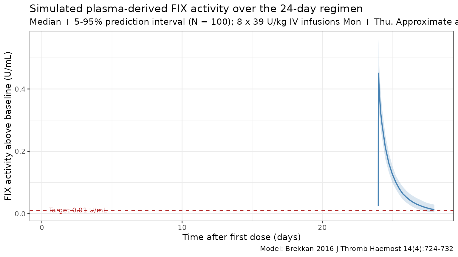

Trough back-check at 96 h after the eighth dose

Brekkan 2016 p. 726 fixes the simulation dose (39 U/kg) by the criterion that “it resulted in a trough FIX activity level of 0.01 U mL-1 in a patient with a body weight of 70 kg.” The check below evaluates that trough in the typical-value simulation (zeroRe() + rbase = 0) for a 70 kg subject.

mod_typ_70 <- rxode2::zeroRe(mod)
#> ℹ parameter labels from comments will be replaced by 'label()'
events_70 <- build_events(tibble(ID = 1L, WT = 70, treatment = "70 kg ref"))
sim_typ_70 <- rxode2::rxSolve(
  mod_typ_70, events = events_70,
  params = c(lrbase = -Inf),
  returnType = "data.frame"
)
#> ℹ omega/sigma items treated as zero: 'etalcl', 'etalvc', 'etalvp', 'etalvp2', 'etalrbase'

trough_row <- sim_typ_70[sim_typ_70$time == last_dose + 96, ]
trough_val <- trough_row$Cc

knitr::kable(
  data.frame(
    quantity         = c("Trough at 96 h after dose 8 (typical, 70 kg, 39 U/kg)",
                         "Brekkan 2016 target trough"),
    value_U_per_mL   = c(round(trough_val, 4), 0.01)
  ),
  caption = "Typical-value trough check for the dose-individualisation design.",
  align   = c("l", "r")
)

Typical-value trough check for the dose-individualisation design.

quantity	value_U_per_mL
Trough at 96 h after dose 8 (typical, 70 kg, 39 U/kg)	0.0127
Brekkan 2016 target trough	0.0100

Typical CL and Vss back-check

Brekkan 2016 Table 2 reports the structural parameters for a typical 70 kg subject. Reproducing those numbers from a single-bolus typical-value simulation is the simplest self-consistency check (Vss = V1 + V2 + V3).

ev_ref <- rxode2::et(amt = 50 * 70, time = 0, cmt = "central") |>
  rxode2::et(0)
sim_ref <- rxode2::rxSolve(
  mod_typ, events = ev_ref,
  params = c(WT = 70, lrbase = -Inf),
  returnType = "data.frame"
)
#> ℹ omega/sigma items treated as zero: 'etalcl', 'etalvc', 'etalvp', 'etalvp2', 'etalrbase'

ref_pars <- sim_ref[1, c("cl", "vc", "q", "vp", "q2", "vp2"), drop = FALSE]
ref_pars$Vss <- ref_pars$vc + ref_pars$vp + ref_pars$vp2

knitr::kable(
  ref_pars,
  caption = "Typical-value PK parameters for the reference 70 kg patient (mL, mL/h).",
  digits  = c(2, 1, 2, 2, 2, 2, 1)
)

Typical-value PK parameters for the reference 70 kg patient (mL, mL/h).

cl	vc	q	vp	q2	vp2	Vss
319.8	5922	1049	828.9	160.4	2234	8984.9

The model returns CL = 319.8 mL/h, V1 = 5922 mL, Q2 = 1049 mL/h, V2 = 828.9 mL, Q3 = 160.4 mL/h, V3 = 2234 mL, and Vss = V1 + V2 + V3 = 8985 mL — matching the values reported in Brekkan 2016 Table 2 (CL = 319.8 mL/h, V1 = 5922 mL, Q2 = 1049 mL/h, V2 = 828.9 mL, Q3 = 160.4 mL/h, V3 = 2234 mL, Vss = 8985 mL).

PKNCA validation: single-dose summary

Brekkan 2016 does not tabulate single-dose NCA parameters directly; the paper’s quantitative results are framed in terms of dose-individualisation performance rather than NCA descriptors. The PKNCA summary below provides the standard NCA descriptors (Cmax, AUC0-inf, terminal half-life) on a single-dose schedule for context.

single_events <- cohort |>
  mutate(AMT = WT * 50) |>
  tidyr::crossing(TIME = c(0, c(0.1, 0.5, 1, 2, 4, 6, 12, 18, 24,
                                30, 36, 42, 48, 54, 60, 66, 72,
                                78, 84, 90, 96, 120, 144, 168, 240, 336))) |>
  mutate(
    EVID = if_else(TIME == 0, 1L, 0L),
    AMT  = if_else(TIME == 0, AMT, NA_real_),
    RATE = if_else(TIME == 0, AMT / infusion_h, NA_real_),
    CMT  = "central",
    DV   = NA_real_
  ) |>
  arrange(ID, TIME, desc(EVID)) |>
  as.data.frame()

sim_single <- rxode2::rxSolve(
  mod, events = single_events,
  params = c(lrbase = -Inf),
  keep   = c("treatment", "WT"),
  returnType = "data.frame"
)
#> ℹ parameter labels from comments will be replaced by 'label()'
sim_single <- sim_single[sim_single$time >= 0, ]

sim_nca <- sim_single |>
  filter(!is.na(Cc)) |>
  select(id, time, Cc, treatment)

# Guarantee a time=0 row per (id, treatment); IV bolus pre-dose Cc=0.
sim_nca <- bind_rows(
  sim_nca,
  sim_nca |> distinct(id, treatment) |> mutate(time = 0, Cc = 0)
) |>
  distinct(id, treatment, time, .keep_all = TRUE) |>
  arrange(id, treatment, time)

dose_df <- single_events |>
  filter(EVID == 1) |>
  transmute(id = ID, time = TIME, amt = AMT, treatment)

conc_obj <- PKNCA::PKNCAconc(sim_nca, Cc ~ time | treatment + id,
                             concu = "U/mL",
                             timeu = "h")
dose_obj <- PKNCA::PKNCAdose(dose_df, amt ~ time | treatment + id,
                             doseu = "U")

intervals <- data.frame(
  start      = 0,
  end        = Inf,
  cmax       = TRUE,
  tmax       = TRUE,
  aucinf.obs = TRUE,
  half.life  = TRUE,
  clast.obs  = TRUE,
  lambda.z   = TRUE
)

nca_res <- PKNCA::pk.nca(PKNCA::PKNCAdata(conc_obj, dose_obj,
                                          intervals = intervals))
nca_tbl <- as.data.frame(nca_res$result)

summary_by_param <- function(param) {
  nca_tbl |>
    filter(PPTESTCD == param) |>
    group_by(treatment) |>
    summarise(
      n        = sum(!is.na(PPORRES)),
      median   = stats::median(PPORRES, na.rm = TRUE),
      q05      = stats::quantile(PPORRES, 0.05, na.rm = TRUE),
      q95      = stats::quantile(PPORRES, 0.95, na.rm = TRUE),
      .groups  = "drop"
    )
}

nca_summary <- bind_rows(
  summary_by_param("cmax")       |> mutate(parameter = "Cmax (U/mL)"),
  summary_by_param("tmax")       |> mutate(parameter = "Tmax (h)"),
  summary_by_param("aucinf.obs") |> mutate(parameter = "AUC0-inf (U*h/mL)"),
  summary_by_param("half.life")  |> mutate(parameter = "Terminal half-life (h)")
) |>
  select(parameter, n, median, q05, q95)

knitr::kable(
  nca_summary,
  caption = "Simulated plasma-derived FIX NCA after a single 50 U/kg IV infusion.",
  digits  = c(0, 0, 3, 3, 3)
)

Simulated plasma-derived FIX NCA after a single 50 U/kg IV infusion.

parameter	n	median	q05	q95
Cmax (U/mL)	100	0.519	0.416	0.696
Tmax (h)	100	0.500	0.500	0.500
AUC0-inf (U*h/mL)	100	10.585	8.500	12.911
Terminal half-life (h)	100	22.503	13.328	56.924

Errata

No published erratum was located for Brekkan 2016 (J Thromb Haemost 2016;14(4):724-732). The packaged parameter values are taken from Brekkan 2016 Table 2 (final model), which is internally consistent with the equations on p. 725 and the simulation design on p. 726.

Assumptions and deviations

• Inter-occasion variability omitted. Brekkan 2016 estimated IOV on CL (21.4% CV) and V1 (20.1% CV) with a correlation of 0.902 between the two random effects (Table 2). The static library model has no occasion variable, so IOV is not implemented as a separate eta. For Bayesian forecasting use cases that explicitly model occasions, the IOV variances (omega^2_IOV_CL = 0.214^2 = 0.045796 and omega^2_IOV_V1 = 0.201^2 = 0.040401, covariance 0.902 * 0.214 * 0.201 = 0.038804) can be added on top of the packaged IIV.
• Inter-individual variability convention. Brekkan 2016 does not state the IIV definition formula directly in the Table 2 footnote, but the related factor IX papers from the same modelling lineage (Diao 2014 Table 3 footnote; Koopman 2023 Table 2 footnote) both define the IIV column as sqrt(variance) * 100, i.e. the reported value equals the SD of the log-scale eta directly. The packaged variances were computed with omega^2 = (reported_value)^2 and covariances as corr * sqrt(var1) * sqrt(var2) to match this convention. For the small IIVs (x_CL = 0.127, x_V1 = 0.157) the two interpretations (omega^2 = reported^2 vs. omega^2 = log(reported^2 + 1)) differ by less than 1%; for the large IIV on V3 (x_V3 = 1.020) they differ by ~30%, which is the dominant uncertainty in any user-facing simulation of the terminal-phase variability.
• No IIV on Q2 or Q3. Brekkan 2016 retained five fewer parameters than the original Berntorp model after model simplification, dropping IIV on Q2 and Q3 (Results, p. 727: “the original model could be reduced by four parameters related to the IIV part”). The packaged model carries no etalq or etalq2.
• Endogenous baseline FIX activity. Brekkan 2016 fits the baseline FIX activity as a structural parameter rather than baseline-correcting the observations. The model output Cc = central / vc + rbase therefore represents total measured FIX activity (exogenous-attributable + endogenous baseline). To represent severe haemophilia B (the simulation design of Brekkan 2016 p. 726), set rbase = 0 by passing params = c(lrbase = -Inf) to rxSolve() (as used in the simulations in this vignette). To represent a patient with moderate haemophilia B and endogenous activity, leave lrbase at its default value.
• Allometric exponents fixed at theoretical values. Brekkan 2016 Methods p. 725 fixes the body weight exponent at 1 for volumes and 0.75 for intercompartmental CL parameters; Results p. 727 fixes the exponent on CL at 0.75 after evaluating three approaches (estimated, fixed at 1.26 from the original Berntorp model, fixed at 0.75) that all gave similar fits. The packaged model() block multiplies CL, Q2, Q3 by (WT / 70)^0.75 and V1, V2, V3 by (WT / 70)^1.00.
• FIX product covariate omitted. Brekkan 2016 tested seven plasma- derived FIX products as a categorical covariate on CL. The likelihood- ratio test was statistically significant (P < 0.01, df = 6) but the largest deviation from AlphaNine was within +/- 20% of the typical CL (range 252-378 mL/h vs. 315 mL/h reference), so the clinical-significance criterion was not met and the product effect was dropped from the final model (Brekkan 2016 Results, p. 727). The Discussion notes the final model “should be used with caution to describe the FIX activity following administration of products that are not plasma-derived.”
• Age covariate omitted. Brekkan 2016 tested age as a fractional-change effect on CL (Equation 2 in the paper) and found it not statistically significant. The Discussion notes that incorporating body weight in the model explains part of the variability related to age.
• Virtual cohort. Body weight was sampled from a log-normal distribution centred at the cohort mean (66.8 kg) and capped at a plausible adult haemophilia B range (45-110 kg). The empirical body weight distribution in Brekkan 2016 (per-study means 61.0-69.7 kg, overall SD 13.5 kg) is approximated, not exactly reproduced.
• Haemophilia B is X-linked recessive, so the development cohort and the virtual cohort here are essentially all male (sex_female_pct = 0 in the population metadata). The model has no sex covariate.