Receptor rebound with homeostatic feedback in TMDD (Aston 2017)
Source:vignettes/articles/Aston_2017_receptor_rebound.Rmd
Aston_2017_receptor_rebound.RmdModel and source
Aston et al. (2017) is the second of two mathematical-analysis papers on receptor rebound - a post-dose rise of free target above its own pre-dose baseline. Paper I (Aston et al. 2014) showed that the basic target-mediated drug disposition (TMDD) model rebounds if and only if the drug-target complex is eliminated more slowly than both the drug and the target. Paper II adds homeostatic feedback on the target synthesis rate and shows that a slow feedback moderator produces rebound for any combination of elimination rates.
Section 7 works the theory through two fully parameterised examples, and each is packaged here as its own model file.
mod_oma <- readModelDb("Aston_2017_omalizumab_qsp")
mod_efa <- readModelDb("Aston_2017_efalizumab_qsp")- Citation: Aston PJ, Derks G, Agoram BM, van der Graaf PH. A mathematical analysis of rebound in a target-mediated drug disposition model: II. With feedback. J Math Biol. 2017;75(1):33-84. doi:10.1007/s00285-016-1073-6. Companion model from the same paper: modellib(‘Aston_2017_efalizumab_qsp’). The omalizumab parameter values are attributed by Aston et al. to Sun T (2001), poster, Advanced Methods of PKPD Systems Analysis, Los Angeles, and Agoram BM, Martin SW, van der Graaf PH, Drug Discov Today. 2007;12(23-24):1018-1024, doi:10.1016/j.drudis.2007.10.002; they are reproduced in full in Sect. 7.1 of the present paper.
- Article: https://doi.org/10.1007/s00285-016-1073-6
- Open access at Europe PMC: https://europepmc.org/article/MED/27833213
Example 1 – Aston_2017_omalizumab_qsp.
QSP. Target-mediated drug disposition (TMDD) with HOMEOSTATIC FEEDBACK
on the free-receptor synthesis rate, parameterised for the anti-IgE mAb
omalizumab (Example 1, Sect. 7.1 of Aston et al. 2017). The classical
Levy / Mager-Jusko one-compartment TMDD system (free ligand L, free
receptor R, ligand-receptor complex P) is extended with a fourth state,
a feedback moderator F that scales the zero-order receptor synthesis
rate and relaxes first-order toward a feedback function H(R) of the
free-receptor level. The paper’s result is that the moderator’s response
SPEED decides whether free receptor rebounds above baseline after a
dose: with these omalizumab parameters ke(L) < ke(P), so the
no-feedback and fast-feedback (direct, quasi-equilibrium) limits can
never rebound, yet a slow moderator produces a rebound peaking near 117%
of baseline. ktol is the paper’s swept quantity (alpha); its default is
the analytic bound of Theorem 5.12, which is also close to the
maximum-rebound alpha of Fig. 10. Deterministic illustration: no
subjects were fitted, so there is no inter-individual variability and no
residual-error model.
Example 2 – Aston_2017_efalizumab_qsp.
QSP. Five-state PK / receptor / feedback model of efalizumab and CD11a
down-modulation in moderate-to-severe psoriasis (Example 2, Sect. 7.2 of
Aston et al. 2017, reproducing the model of Ng et al. 2005). A
two-compartment PK backbone with first-order subcutaneous absorption and
PARALLEL linear plus Michaelis-Menten elimination drives saturable
down-modulation of the total CD11a on the T-cell surface; the CD11a
production rate is itself a dynamic state that relaxes toward a
hyperbolic, negative-feedback function of the CD11a level. That slow
feedback is what makes total CD11a REBOUND to about 140% of baseline
around day 50 after a single 3 mg/kg intravenous dose, which the same
model without feedback does not do. The whole model is BODY-WEIGHT
NORMALISED: every drug amount is per kg and Vc is 64.3 mL/kg. CD11a is
carried as a percentage of its own baseline, so total_target starts at
100. Deterministic illustration: no subjects were fitted in Aston et
al., so there is no inter-individual variability and no residual-error
model.
Population
Neither example is a fit. Aston et al. fitted no subject-level data anywhere in the paper; Section 7 re-simulates two previously published models in order to test the paper’s analytic rebound criteria against them.
-
Example 1 uses literature parameter values for the
anti-IgE monoclonal antibody omalizumab, attributed in Section 7.1 to
Sun (2001) and Agoram et al. (2007). There is no study population, no
inter-individual variability and no residual-error model, so every
parameter is encoded with
fixed(). -
Example 2 reproduces the efalizumab model of Ng et
al. (2005), developed in patients with moderate-to-severe plaque
psoriasis. The subject count and demographics live in Ng et al. (2005),
which was not available when this model was built, so
population$n_subjectsis leftNArather than guessed. The model is body-weight normalised throughout (Vc= 64.3 mL/kg, dose in mg/kg), and CD11a is expressed as a percentage of its own baseline.
The same information is available programmatically via each model’s
population metadata,
e.g. readModelDb("Aston_2017_efalizumab_qsp")()$population.
Source trace
Every value below is transcribed from Section 7 of Aston et
al. (2017); the per-parameter origin is also recorded as an in-file
comment beside each ini() entry.
Example 1 – omalizumab TMDD with a feedback moderator
| Equation / parameter | Value | Source location |
|---|---|---|
d/dt(central), d/dt(complex),
d/dt(target), d/dt(moderator1)
|
n/a | Eqs. (11)-(14), Sect. 3 |
Initial conditions target(0) = R0,
complex(0) = 0, moderator1(0) = 1
|
n/a | Eq. (4) plus the sentence following Eq. (14) |
Feedback function H(R) = 1 + H0 * (R0 - R)
|
H0 = 1 /nM |
Eq. (34) with the H0 = 1 of Sect. 7.1 |
lkel (Aston ke(L)) |
0.024 /day | Sect. 7.1 |
kint (Aston ke(P)) |
0.201 /day | Sect. 7.1 |
kdeg (Aston kout) |
0.823 /day | Sect. 7.1 |
bl_target (Aston R0) |
2.688 nM | Sect. 7.1 |
koff |
0.900 /day | Sect. 7.1 |
kon |
0.592 /(nM*day) | Sect. 7.1 |
ksyn (Aston kin = kout * R0) |
2.212224 nM/day, derived in model()
|
Sect. 7.1 |
ktol (Aston alpha) |
0.135 /day | Sect. 7.1, the Theorem 5.12 rebound bound |
sstim_target_moderator1 |
-1 /nM (= -H0) |
Eq. (34); sign flips because the register writes the driver
deviation as driver - baseline
|
Dose L0
|
14.8148 nM | Sect. 7.1 |
Example 2 – efalizumab and CD11a down-modulation
| Equation / parameter | Value | Source location |
|---|---|---|
The five dX/dt equations |
n/a | Sect. 7.2, the unnumbered display following “The model equations proposed in Ng et al. (2005) are” |
Free CD11a = Kmc * Vc * X3 / (Kmc * Vc + X1)
|
n/a | Sect. 7.2, final paragraph |
Baseline steady state
k03max * F^2 + k30 * Kmc03 * F - k30 * Kmc03 = 0
|
n/a | Eq. (72) |
lka |
0.242 /day | Sect. 7.2 (from Ng 2005 Tables II-III) |
lkel (Aston k10) |
0.114 /day | Sect. 7.2 |
lk12 |
0.097 /day | Sect. 7.2 |
lk21 |
0.193 /day | Sect. 7.2 |
kdeg (Aston k30) |
0.444 /day | Sect. 7.2 |
lvc |
64.3 mL/kg | Sect. 7.2 |
lvmax (Aston Vm) |
26.9 ug/kg/day | Sect. 7.2, units corrected – see Errata |
km (Aston Kmc) |
0.033 ug/mL | Sect. 7.2 |
kmax_total_target (Aston Vm2) |
2.16 /day | Sect. 7.2 |
kinmax (Aston k03max) |
334 %CD11a/day | Sect. 7.2 |
lfdepot (Aston Fa) |
0.564 | Sect. 7.2 |
ktol (Aston koff) |
0.0154 /day | Sect. 7.2, Aston’s ten-fold correction – see Errata |
bl_total_target |
100 %CD11a | Fig. 11 axis “%CD11a/baseline”; km_moderator1 (Aston
Kmc03) is derived from it via Eq. (72) – see Errata |
| Dose | 3 mg/kg = 3000 ug/kg IV | Fig. 11 caption |
Example 1 – omalizumab TMDD with a feedback moderator
Analytic anchors
Section 7.1 prints three non-dimensional quantities for this
parameter set. They are closed-form functions of the ini()
values, so reproducing them is an exact transcription check on
kel, kint, kdeg,
kon, koff and bl_target all at
once. The scaling of Eq. (15) and the definitions after Eq. (19) are
and lambda1 is the eigenvalue closest to zero of the
linearisation of the (x, z) sub-system about the drug-free
steady state.
p_oma <- rxode2::rxode(mod_oma)$theta
oma <- c(
  kel = exp(p_oma[["lkel"]]),
  kint = p_oma[["kint"]],
  kdeg = p_oma[["kdeg"]],
  kon = p_oma[["kon"]],
  koff = p_oma[["koff"]],
  R0 = p_oma[["bl_target"]]
)

scale_oma <- oma[["kon"]] * oma[["R0"]]
k1 <- oma[["kel"]] / scale_oma
k2 <- oma[["koff"]] / scale_oma
k3 <- oma[["kdeg"]] / scale_oma
k4 <- oma[["kint"]] / scale_oma

# Linearisation of Eqs. (16)-(17) about (x, z) = (0, 0) at y = 1. The
# dimensionless mu = R0 / L0 cancels out of the characteristic polynomial.
jac_xz <- matrix(c(-(k1 + 1), k2, 1, -(k2 + k4)), nrow = 2, byrow = TRUE)
lambda1 <- max(Re(eigen(jac_xz)$values))

e1_anchor <- tibble::tibble(
  quantity = c("k3", "k4", "lambda1"),
  computed = c(k3, k4, lambda1),
  published = c(0.517, 0.126, -0.084)
)
knitr::kable(e1_anchor, digits = 4,
caption = "Section 7.1 non-dimensional anchors, computed vs published.")| quantity | computed | published |
|---|---|---|
| k3 | 0.5172 | 0.517 |
| k4 | 0.1263 | 0.126 |
| lambda1 | -0.0843 | -0.084 |
# Deterministic, closed-form quantities: assert tightly. The published values
# carry three decimals, so half a unit in the last place is the exact tolerance.
stopifnot(
  abs(k3 - 0.517) < 5e-4,
  abs(k4 - 0.126) < 5e-4,
  abs(lambda1 - (-0.084)) < 5e-4
)

# Section 7.1: "These parameter values have ke(L) < ke(P) and so no rebound
# will occur when there is no feedback or in the case of direct feedback."
stopifnot(oma[["kel"]] < oma[["kint"]])
Steady-state hold
With no dose the system must sit exactly on the drug-free steady
state of Eq. (4): free receptor at R0, complex at zero,
moderator at 1.
ev_hold <- rxode2::et(seq(0, 400, by = 10))
hold_oma <- rxode2::rxSolve(mod_oma, ev_hold, returnType = "data.frame")

stopifnot(
  max(abs(hold_oma$targetRatio - 1)) < 1e-8,
  max(abs(hold_oma$moderator1 - 1)) < 1e-8,
  max(abs(hold_oma$complex)) < 1e-8
)
cat(sprintf("Undosed drift over 400 days: max |R/R0 - 1| = %.2e\n",
            max(abs(hold_oma$targetRatio - 1))))
#> Undosed drift over 400 days: max |R/R0 - 1| = 0.00e+00
Figure 10 – rebound magnitude and timing against the feedback speed
Figure 10 sweeps the moderator response rate alpha and
plots the relative rebound Rmax / R0 (left) and the time
tmax at which it occurs (right). A single bolus of
L0 = 14.8148 nM is added to the free-ligand state.
# Deterministic solves, one per alpha; no cohort and no random effects, so a
# single "subject" is the whole simulation.
sweep_alpha <- function(alpha, tend = 400, n = 4001) {
  ev <- rxode2::et(amt = 14.8148, cmt = "central") |>
    rxode2::et(seq(0, tend, length.out = n))
  s <- rxode2::rxSolve(mod_oma, ev, params = c(ktol = alpha),
                       returnType = "data.frame")
  s <- s[s$time > 0, ]
  i <- which.max(s$targetRatio)
  tibble::tibble(alpha = alpha, rmax = s$targetRatio[i], tmax = s$time[i])
}

alphas <- c(0, 0.005, 0.01, 0.02, 0.04, 0.06, 0.08, 0.10, 0.12, 0.135, 0.15,
            0.20, 0.25, 0.30, 0.40, 0.50, 0.60, 0.70, 0.80, 0.90, 0.95, 0.98,
            1.00, 1.10, 1.20)
sweep <- dplyr::bind_rows(lapply(alphas, sweep_alpha))

# alpha = 0 is the no-feedback limit: the maximum of R is just the asymptotic
# return to baseline, which lands at the far end of the integration window and
# is not a rebound. Flag it so the tmax panel is not misread.
sweep <- sweep |>
  dplyr::mutate(rebound = rmax > 1 + 1e-6)
# Replicates Figure 10 of Aston et al. (2017).
p_left <- sweep |>
  ggplot(aes(alpha, rmax)) +
  geom_line() +
  geom_hline(yintercept = 1, linetype = "dashed") +
  labs(x = "alpha (1/day)", y = "Rmax / R0",
       title = "Figure 10 (left) - relative rebound magnitude")

p_right <- sweep |>
  dplyr::filter(rebound) |>
  ggplot(aes(alpha, tmax)) +
  geom_line() +
  labs(x = "alpha (1/day)", y = "tmax (day)",
       title = "Figure 10 (right) - time of maximum rebound")

print(p_left)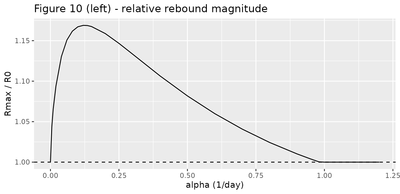
print(p_right)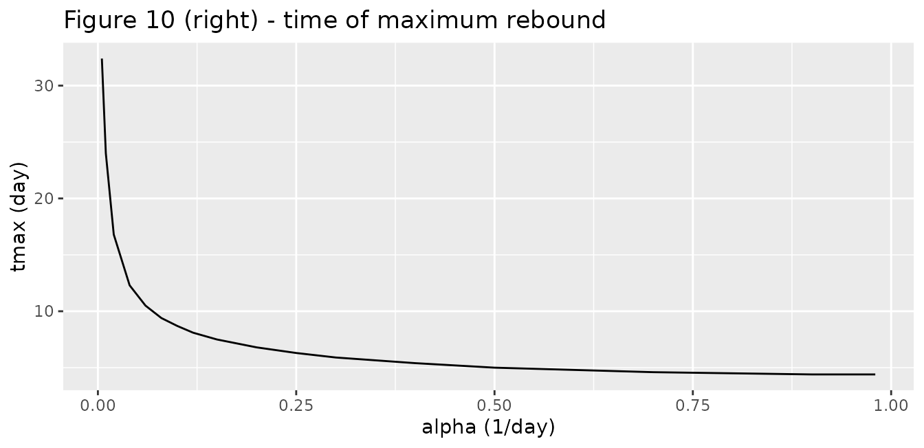
peak <- sweep$rmax[which.max(sweep$rmax)]
peak_alpha <- sweep$alpha[which.max(sweep$rmax)]
last_rebound_alpha <- max(sweep$alpha[sweep$rebound])

cat(sprintf(paste0("Maximum Rmax/R0 = %.4f at alpha = %.3f /day; ",
                   "rebound is lost between alpha = %.2f and %.2f /day\n"),
            peak, peak_alpha, last_rebound_alpha,
            min(sweep$alpha[sweep$alpha > last_rebound_alpha])))
#> Maximum Rmax/R0 = 1.1689 at alpha = 0.120 /day; rebound is lost between alpha = 0.98 and 1.00 /day

stopifnot(
  # Sect. 7.1: no rebound at alpha = 0, and Fig. 3 / Theorem 2.1 agree because
  # ke(L) < ke(P) for this parameter set.
  !sweep$rebound[sweep$alpha == 0],
  # Sect. 7.1: "rebound will happen for alpha < 0.135" (Theorem 5.12 bound).
  all(sweep$rebound[sweep$alpha > 0 & sweep$alpha <= 0.135]),
  # Sect. 7.1: "the rebound ends at approximately alpha = 0.98". The sweep's
  # last rebounding alpha IS 0.98 and the next grid point (1.00) does not
  # rebound; allow one grid step either side so the gate does not depend on
  # the grid chosen here.
  last_rebound_alpha >= 0.90, last_rebound_alpha <= 1.00,
  # Fig. 10 left: the curve peaks just under 1.17, close to the Theorem 5.12
  # bound. Digitised from the published panel, hence the 0.01 window.
  abs(peak - 1.167) < 0.015,
  peak_alpha >= 0.08, peak_alpha <= 0.20,
  # Sect. 7.1: "as alpha -> 0 then tmax -> infinity".
  sweep$tmax[sweep$alpha == 0.005] > sweep$tmax[sweep$alpha == 0.135],
  # Abstract: "for a very fast feedback response ... in a very similar way as
  # for no feedback" - the direct-feedback limit cannot rebound here.
  !sweep$rebound[sweep$alpha == 1.20]
)
Time courses at the default feedback speed
ev_dose <- rxode2::et(amt = 14.8148, cmt = "central") |>
  rxode2::et(seq(0, 60, length.out = 1201))

tc <- dplyr::bind_rows(
  rxode2::rxSolve(mod_oma, ev_dose, params = c(ktol = 0),
                  returnType = "data.frame") |>
    dplyr::mutate(scenario = "alpha = 0 (no feedback)"),
  rxode2::rxSolve(mod_oma, ev_dose, returnType = "data.frame") |>
    dplyr::mutate(scenario = "alpha = 0.135 (slow feedback, default)"),
  rxode2::rxSolve(mod_oma, ev_dose, params = c(ktol = 5),
                  returnType = "data.frame") |>
    dplyr::mutate(scenario = "alpha = 5 (fast feedback)")
)

tc |>
  ggplot(aes(time, 100 * targetRatio, colour = scenario)) +
  geom_line() +
  geom_hline(yintercept = 100, linetype = "dashed") +
  labs(x = "Time (day)", y = "Free receptor (% of baseline)",
       colour = NULL,
       title = "Free receptor after a single 14.8148 nM bolus",
       caption = "Only the slow moderator rebounds above baseline.") +
  theme(legend.position = "bottom")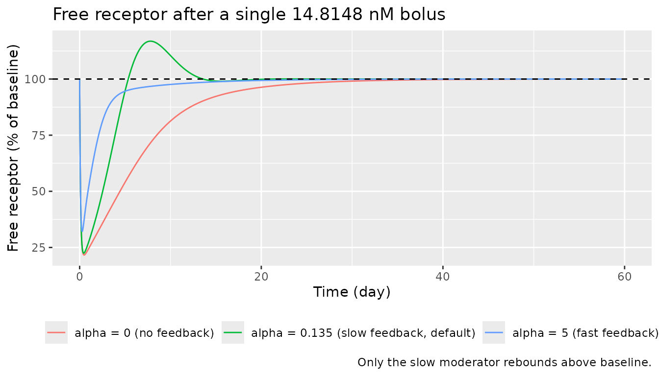
Example 2 – efalizumab and CD11a down-modulation
Deriving the unprinted feedback constant
Every parameter of the Section 7.2 model is printed except
Kmc03, the half-saturation constant of the feedback
function H(X3) = Kmc03 / (Kmc03 + X3). It is not missing
information: X3 is the total CD11a expressed as a
percentage of its own baseline, so the drug-free steady state
is 100 by construction - which is exactly what the Fig. 11 axis
(“%CD11a/baseline”, both panels starting at 100 and the no-feedback
panel returning to it) shows. Given that baseline, Aston’s Eq. (72)
fixes Kmc03 exactly, and the model file derives it inside
model() rather than hard-coding a number.
p_efa <- rxode2::rxode(mod_efa)$theta
efa <- c(
  ka = exp(p_efa[["lka"]]), kel = exp(p_efa[["lkel"]]),
  k12 = exp(p_efa[["lk12"]]), k21 = exp(p_efa[["lk21"]]),
  fdepot = exp(p_efa[["lfdepot"]]), vc = exp(p_efa[["lvc"]]),
  vmax = exp(p_efa[["lvmax"]]), km = p_efa[["km"]],
  kdeg = p_efa[["kdeg"]], kmax = p_efa[["kmax_total_target"]],
  kinmax = p_efa[["kinmax"]], ktol = p_efa[["ktol"]],
  bl = p_efa[["bl_total_target"]]
)

f0 <- efa[["kdeg"]] * efa[["bl"]] / efa[["kinmax"]]
kmc03 <- efa[["kinmax"]] * f0^2 / (efa[["kdeg"]] * (1 - f0))
cat(sprintf("F0 = %.6f, Kmc03 = %.4f %%CD11a\n", f0, kmc03))
#> F0 = 0.132934, Kmc03 = 15.3315 %CD11a

# Eq. (72) must hold at the derived value; this is the inversion's own check.
stopifnot(
  abs(efa[["kinmax"]] * f0^2 + efa[["kdeg"]] * kmc03 * f0 -
        efa[["kdeg"]] * kmc03) < 1e-9
)
The derivation is corroborated below against a number Aston et
al. print but never use to define anything: the slowest eigenvalue of
the feedback block. Only the definitional baseline of 100 reproduces the
published -1.37e-2 at its printed precision.
lambda_fb_for <- function(baseline) {
  f <- efa[["kdeg"]] * baseline / efa[["kinmax"]]
  k3b <- efa[["kdeg"]] / efa[["kmax"]]
  ep <- efa[["ktol"]] / efa[["kmax"]]
  jac <- matrix(c(-k3b, k3b, -ep * (1 - f), -ep), nrow = 2, byrow = TRUE)
  max(Re(eigen(jac)$values))
}

discriminate <- tibble::tibble(
  `assumed baseline %CD11a` = c(80, 100, 120),
  `slowest feedback eigenvalue` = vapply(c(80, 100, 120), lambda_fb_for, numeric(1))
) |>
  dplyr::mutate(`relative error vs published -1.37e-2` =
                  `slowest feedback eigenvalue` / -1.37e-2 - 1)
knitr::kable(discriminate, digits = c(0, 6, 4),
caption = "Only a baseline of 100 %CD11a matches the printed eigenvalue.")| assumed baseline %CD11a | slowest feedback eigenvalue | relative error vs published -1.37e-2 |
|---|---|---|
| 80 | -0.013965 | 0.0194 |
| 100 | -0.013755 | 0.0040 |
| 120 | -0.013545 | -0.0113 |
Analytic anchors
Section 7.2 prints three numbers that depend on the whole parameter
set, including the derived Kmc03. All three are in the
non-dimensional time tau = Vm2 * t. Reproducing them is the
independent corroboration that both the Kmc03 derivation
above and the Vm units correction below are right.
eps <- efa[["ktol"]] / efa[["kmax"]]
k3_efa <- efa[["kdeg"]] / efa[["kmax"]]
h0_efa <- 1 - f0

# Lower 2x2 block of the Jacobian, Eq. (69), with g(y, w) = h(y) - w so that
# g1 = -h'(1) = h0 and g2 = -1.
jac_fb <- matrix(c(-k3_efa, k3_efa, -eps * h0_efa, -eps), nrow = 2, byrow = TRUE)
lambda_fb <- max(Re(eigen(jac_fb)$values))

# 3x3 PK block D_x f1(0, 1): the depot / central / peripheral linearisation at
# zero drug, where the Michaelis-Menten term linearises to Vm / (Kmc * Vc).
jac_pk <- matrix(
  c(-efa[["ka"]], 0, 0,
    efa[["fdepot"]] * efa[["ka"]],
    -(efa[["kel"]] + efa[["k12"]]) - efa[["vmax"]] / (efa[["km"]] * efa[["vc"]]),
    efa[["k21"]],
    0, efa[["k12"]], -efa[["k21"]]),
  nrow = 3, byrow = TRUE
) / efa[["kmax"]]
lambda_pk <- max(Re(eigen(jac_pk)$values))

e2_anchor <- tibble::tibble(
  quantity = c("epsilon = koff / Vm2",
               "slowest eigenvalue, feedback block",
               "slowest eigenvalue, PK block"),
  computed = c(eps, lambda_fb, lambda_pk),
  published = c(7.13e-3, -1.37e-2, -8.87e-2)
)
knitr::kable(e2_anchor, digits = 6,
caption = "Section 7.2 non-dimensional anchors, computed vs published.")| quantity | computed | published |
|---|---|---|
| epsilon = koff / Vm2 | 0.007130 | 0.00713 |
| slowest eigenvalue, feedback block | -0.013755 | -0.01370 |
| slowest eigenvalue, PK block | -0.088669 | -0.08870 |
# Deterministic closed-form quantities again. The published values carry three
# significant figures; 0.6% is half a unit in the last place of the tightest
# of them and still comfortably excludes any competing reading.
stopifnot(
  abs(eps / 7.13e-3 - 1) < 0.006,
  abs(lambda_fb / -1.37e-2 - 1) < 0.006,
  abs(lambda_pk / -8.87e-2 - 1) < 0.006,
  # Sect. 7.2: "0 < epsilon < epsilon_0", i.e. the feedback block is the slow
  # one, which is what makes Theorem 6.1 predict rebound in the total receptor.
  lambda_fb > lambda_pk
)
Steady-state hold
hold_efa <- rxode2::rxSolve(mod_efa, rxode2::et(seq(0, 400, by = 10)),
                            returnType = "data.frame")
stopifnot(
  max(abs(hold_efa$totalCD11a - 100)) < 1e-8,
  max(abs(hold_efa$freeCD11a - 100)) < 1e-8,
  max(abs(hold_efa$Cc)) < 1e-10
)
cat(sprintf("Undosed drift over 400 days: max |CD11a - 100| = %.2e\n",
            max(abs(hold_efa$totalCD11a - 100))))
#> Undosed drift over 400 days: max |CD11a - 100| = 0.00e+00
Figure 11 – CD11a after a single 3 mg/kg intravenous dose
Figure 11 shows total and free CD11a relative to baseline, with
feedback on (left) and off (right). Aston et al. turn the feedback off
by holding X4 constant at its baseline value, which is
ktol = 0 here.
ev_efa <- rxode2::et(amt = 3000, cmt = "central") |>
  rxode2::et(seq(0, 80, length.out = 1601))

sim_efa <- dplyr::bind_rows(
  rxode2::rxSolve(mod_efa, ev_efa, returnType = "data.frame") |>
    dplyr::mutate(scenario = "Efalizumab, with feedback"),
  rxode2::rxSolve(mod_efa, ev_efa, params = c(ktol = 0),
                  returnType = "data.frame") |>
    dplyr::mutate(scenario = "Efalizumab, no feedback")
) |>
  dplyr::mutate(scenario = factor(
    scenario,
    levels = c("Efalizumab, with feedback", "Efalizumab, no feedback")
  ))
# Replicates Figure 11 of Aston et al. (2017).
sim_efa |>
  dplyr::select(time, scenario, totalCD11a, freeCD11a) |>
  tidyr::pivot_longer(c(totalCD11a, freeCD11a),
                      names_to = "species", values_to = "pct") |>
  dplyr::mutate(species = dplyr::recode(species,
                                        totalCD11a = "Total %CD11a",
                                        freeCD11a = "Free %CD11a")) |>
  ggplot(aes(time, pct, colour = species, linetype = species)) +
  geom_line() +
  geom_hline(yintercept = 100, linetype = "dotted") +
  facet_wrap(~scenario) +
  coord_cartesian(ylim = c(0, 150)) +
  labs(x = "Time (day)", y = "%CD11a / baseline", colour = NULL, linetype = NULL,
       title = "Figure 11 - CD11a after a single 3 mg/kg IV dose of efalizumab",
       caption = "Replicates Figure 11 of Aston et al. (2017).") +
  theme(legend.position = "bottom")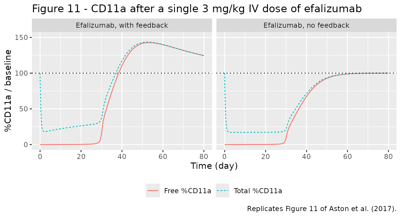
# Base subsetting rather than dplyr::filter(): the post-dose window is a plain
# row selection, and keeping `filter(..., time > 0)` out of the file avoids
# confusing it with a PKNCA input filter (which must never drop time = 0).
fb <- sim_efa[sim_efa$scenario == "Efalizumab, with feedback" & sim_efa$time > 0, ]
nofb <- sim_efa[sim_efa$scenario == "Efalizumab, no feedback" & sim_efa$time > 0, ]

i_pk <- which.max(fb$totalCD11a)
summary_11 <- tibble::tibble(
  quantity = c("peak total %CD11a, with feedback",
               "day of the peak, with feedback",
               "trough total %CD11a, with feedback",
               "peak free %CD11a, with feedback",
               "peak total %CD11a, no feedback"),
  value = c(fb$totalCD11a[i_pk], fb$time[i_pk], min(fb$totalCD11a),
            max(fb$freeCD11a), max(nofb$totalCD11a))
)
knitr::kable(summary_11, digits = 1,
caption = "Figure 11 summary statistics from the packaged model.")| quantity | value |
|---|---|
| peak total %CD11a, with feedback | 143.5 |
| day of the peak, with feedback | 52.5 |
| trough total %CD11a, with feedback | 18.1 |
| peak free %CD11a, with feedback | 142.7 |
| peak total %CD11a, no feedback | 100.0 |
stopifnot(
  # Abstract: "a significant rebound (about 140% of baseline) will occur if
  # feedback is included"; Sect. 8: "an increase of over 40% of baseline".
  fb$totalCD11a[i_pk] > 140, fb$totalCD11a[i_pk] < 148,
  # Fig. 11 left: the peak sits at roughly day 50.
  fb$time[i_pk] > 45, fb$time[i_pk] < 58,
  # Fig. 11 left: total CD11a is driven well below baseline first.
  min(fb$totalCD11a) < 25,
  # Sect. 7.2 final paragraph: once X1 is depleted the free receptor is "very
  # similar to X3 and so will also rebound".
  abs(max(fb$freeCD11a) - fb$totalCD11a[i_pk]) < 2,
  max(fb$freeCD11a) > 140,
  # Sect. 7.2: "without feedback there is no rebound".
  max(nofb$totalCD11a) <= 100 + 1e-6,
  # ... and the no-feedback arm does return to baseline within the window.
  nofb$totalCD11a[nrow(nofb)] > 99
)
PKNCA – efalizumab exposure
Aston et al. report no non-compartmental parameters, so there is no
published NCA table to compare against and no
ncaComparisonTable() here. The block below is a descriptive
exposure summary for the Figure 11 regimen, computed with PKNCA rather
than an inline trapezoidal rule.
The concentration-time profile is truncated at day 40. Efalizumab’s clearance is saturable, so clearance rises as concentration falls and the drug is gone by roughly day 35; integrating past that point only accumulates solver noise.
# Select the feedback arm and truncate the window FIRST, so that the only
# filter standing between the simulation and PKNCA is `!is.na(Cc)`.
sim_window <- sim_efa[sim_efa$scenario == "Efalizumab, with feedback" &
                        sim_efa$time <= 40, ]
sim_window$id <- 1L
sim_window$treatment <- "3 mg/kg IV"

sim_nca <- sim_window |>
  dplyr::filter(!is.na(Cc)) |>
  dplyr::select(id, time, Cc, treatment)

# Guarantee a time = 0 row so PKNCA can anchor AUC0-*; this is an IV bolus, so
# the solve already provides one and the distinct() below keeps it.
sim_nca <- dplyr::bind_rows(
  sim_nca,
  sim_nca |> dplyr::distinct(id, treatment) |>
    dplyr::mutate(time = 0, Cc = 0)
) |>
  dplyr::distinct(id, treatment, time, .keep_all = TRUE) |>
  dplyr::arrange(id, treatment, time)

stopifnot(all(sim_nca$Cc >= 0), any(sim_nca$time == 0))

conc_obj <- PKNCA::PKNCAconc(sim_nca, Cc ~ time | treatment + id)

dose_df <- tibble::tibble(id = 1L, time = 0, amt = 3000, treatment = "3 mg/kg IV")
dose_obj <- PKNCA::PKNCAdose(dose_df, amt ~ time | treatment + id)

intervals <- data.frame(
  start = 0, end = 40,
  cmax = TRUE, tmax = TRUE, auclast = TRUE, half.life = TRUE
)

nca_res <- PKNCA::pk.nca(PKNCA::PKNCAdata(conc_obj, dose_obj,
                                          intervals = intervals))

nca_tab <- as.data.frame(nca_res) |>
  dplyr::select(treatment, PPTESTCD, PPORRES) |>
  tidyr::pivot_wider(names_from = PPTESTCD, values_from = PPORRES)

nca_tab |>
  dplyr::select(treatment, cmax, tmax, auclast, half.life) |>
  dplyr::rename(
    "Regimen" = treatment,
    "Cmax (ug/mL)" = cmax,
    "Tmax (day)" = tmax,
    "AUClast (ug*day/mL)" = auclast,
    "t1/2 (day)" = half.life
  ) |>
  knitr::kable(digits = 2,
caption = "PKNCA summary of the simulated 3 mg/kg IV profile.")| Regimen | Cmax (ug/mL) | Tmax (day) | AUClast (ug*day/mL) | t1/2 (day) |
|---|---|---|---|---|
| 3 mg/kg IV | 46.66 | 0 | 293.58 | 3.3 |
# Cmax after an IV bolus into a per-kg central volume is exactly dose / Vc.
cmax_expected <- 3000 / efa[["vc"]]
cat(sprintf("Cmax expected from dose / Vc = %.1f ug/mL\n", cmax_expected))
#> Cmax expected from dose / Vc = 46.7 ug/mL
stopifnot(
  abs(nca_tab$cmax / cmax_expected - 1) < 0.01,
  nca_tab$tmax == 0,
  # Saturable elimination: the apparent terminal half-life must be much shorter
  # than the linear-only half-life of log(2) / k10 = 6.1 days.
  nca_tab$half.life < log(2) / efa[["kel"]]
)
Assumptions, deviations and errata
-
Kmc03is derived, not transcribed. Aston et al. print eleven of the twelve Section 7.2 parameters but never printKmc03. Ng et al. (2005), where it originates, is not open access and was not available when this model was built. Rather than guess it, the model file parameterises the CD11a pool by its baseline,bl_total_target = 100%CD11a - a value that is not an assumption but the definition of an endpoint reported as a percentage of baseline, and which the Fig. 11 axis displays directly. Eq. (72) then determinesKmc03 = 15.33%CD11a exactly. Two independent checks corroborate it. First, the paper’s printed slowest feedback-block eigenvalue of-1.37e-2, which this value reproduces as-1.3755e-2, a 0.4% error, against roughly 1.9% and 1.1% for the nearest competing baselines of 80 and 120 %CD11a - the discriminating table is computed above. Second, the Figure 11 time course itself, which the model reproduces in peak height, peak timing and trough depth. If Ng et al. (2005) is later acquired, the printedKmc03should be checked against 15.33. -
Vmis printed with the wrong units. Section 7.2 givesVm = 26.9 ug/mL.Vmis the saturating maximum of a term added todX1/dt, so it must carry amount-per-time units, here ug/kg/day; a concentration cannot appear there. The number 26.9 is confirmed by the paper’s own printed PK-block eigenvalue of-8.87e-2, which the model reproduces as-8.8669e-2usingVm / (Kmc * Vc) = 26.9 / 2.1219 = 12.68/day. The model file keeps 26.9 and corrects the units in thelabel(). -
koffuses Aston’s corrected value, not Ng’s printed one. Section 7.2 states that Ng et al.’s printedkoff = 0.00154/day did not reproduce their own Figure 3B and that0.0154/day did.0.0154is what Aston et al. use for Figure 11 and for the printedepsilon = 7.13e-3, so it is what the model encodes. Settingktol = 0.00154recovers the smaller rebound (about 110% of baseline) that Aston reports for the uncorrected value. Aston also notes that neither value reconcileskoff / konwith the affinity of 0.033 ug/mL that Ng et al. report; that discrepancy is unresolved in the source and is inherited here. -
alphais a swept quantity, not an estimate. Example 1’sktolhas no fitted value anywhere. Its default, 0.135 /day, is the analytic bound quoted in Section 7.1 (“rebound will happen for alpha < 0.135”), which also sits close to the numerical maximum of Figure 10. Any other value in(0, 0.98)reproduces a rebound of the magnitude that figure shows. -
sstim_target_moderator1carries the opposite sign to Aston’sH0. The canonicalsstim_<driver>_<target>family is written as1 + sstim * (driver - driver_baseline)whereas Eq. (34) is written as1 + H0 * (R0 - R). The encoded value is therefore-H0 = -1/nM. The negative sign is the correct reading of a negative feedback. -
No variability of any kind. Neither example fits
subject-level data, so there is no inter-individual variability and no
residual-error model anywhere in the source. Both model files set
propSd <- fixed(0)rather than inventing a variance;rxSolveoutput is therefore the typical-value prediction and every assertion in this vignette is deterministic and tight. -
Example 1’s nonlinear feedback branch is not
exercised. Eq. (34) has a nonlinear branch
H1(R)forR > R0 + beta/H0. Section 7.1 states the rebound here is small enough that it is never reached, and the model file implements only the linear branch. The Figure 10 peak ofRmax/R0 = 1.169puts the free receptor at 3.14 nM against a branch point atR0 + 1/H0 = 3.69nM, so the statement holds throughout the swept range. -
Population demographics for Example 2 are
unavailable. They are reported in Ng et al. (2005), which was
not available;
n_subjectsandn_studiesare leftNArather than guessed.