MBG453 (Xu 2023)

Model and source

• Citation: Xu S, Zhang N, Rinne ML, Sun H, Stein AM. Sabatolimab (MBG453) model-informed drug development for dose selection in patients with myelodysplastic syndrome/acute myeloid leukemia and solid tumors. CPT Pharmacometrics Syst Pharmacol. 2023;12(11):1653-1665. doi:10.1002/psp4.12962
• Description: Two-compartment population PK model for sabatolimab (MBG453, anti-TIM-3 IgG4) with parallel linear and Michaelis-Menten elimination from the central compartment, fit to pooled adult patients with advanced solid tumors and hematologic malignancies (Xu 2023).
• Article: https://doi.org/10.1002/psp4.12962
• Supplement (figures, tables, Monolix appendices): published alongside the article in CPT:PSP 2023;12(11) supporting information.

Population

The Xu 2023 PopPK analysis pooled 444 adults from two phase I / Ib trials of sabatolimab (MBG453), an anti-TIM-3 IgG4 antibody: 252 patients with advanced or metastatic solid tumors (NCT02608268) and 192 patients with hematologic malignancies (NCT03066648) – AML, MDS (including intermediate-, high-, and very high-risk per Revised IPSS), or CMML, all ineligible for intensive chemotherapy. Eligibility required age >= 18 years and ECOG performance status 0-2. Sabatolimab was administered as a 30-minute IV infusion at 20-1200 mg Q2W or 80-1200 mg Q4W, alone or in combination with spartalizumab (anti-PD-1, PDR001) and / or hypomethylating agents (decitabine or azacitidine). Treatment-arm composition: 159 sabatolimab monotherapy, 130 sabatolimab + spartalizumab, 55 sabatolimab + azacitidine, and 100 sabatolimab + decitabine +/- spartalizumab.

The hematologic-malignancy cohort was older (median age 71-72.5 years across treatment arms; Table S1) and predominantly Caucasian (68.9-87.9% across arms; the remainder Asian, Black, Other, or Unknown) with ~40% female. The published main paper does not report median baseline weight; the model centers the WT effect on a working reference of 75 kg (see “Assumptions and deviations” below).

The same population metadata is available programmatically via readModelDb("Xu_2023_MBG453")$population.

Source trace

Every parameter’s origin is recorded in-line in inst/modeldb/specificDrugs/Xu_2023_MBG453.R. The table below collects the per-parameter and per-equation provenance for review. Page numbers refer to the published article.

Equation / parameter	Value	Source location
lcl (CL, L/day)	log(0.0103 x 24)	Xu 2023 Table 1, p1660 (CL = 0.0103 L/h)
lvc (V, L)	log(3.59)	Xu 2023 Table 1, p1660 (V = 3.59 L)
lq (Q, L/day)	log(0.0353 x 24)	Xu 2023 Table 1, p1660 (Q = 0.0353 L/h)
lvp (V2, L)	log(2.38)	Xu 2023 Table 1, p1660 (V2 = 2.38 L)
lvmax (Vm, (ug/mL)/day)	log(0.0197 x 24)	Xu 2023 Table 1, p1660 (Vm = 0.0197 ug/mL/h)
lkm (Km, ug/mL, FIXED)	log(0.074)	Xu 2023 Table 1, p1660 footnote a (Km = 0.5 nM = 0.074 ug/mL FIXED)
e_wt_cl (allometric WT on CL)	0.743	Xu 2023 Table 1 row beta_CL,WT0; Eq. on p1657
e_wt_vc (allometric WT on V)	0.770	Xu 2023 Table 1 row beta_V,WT0; Eq. on p1657
e_wt_vp (allometric WT on V2)	0.597	Xu 2023 Table 1 row beta_V2,WT0; Eq. on p1657
e_dis_aml_cl	-0.0146	Xu 2023 Table 1 row beta_CL,AML (NS p = 0.801)
e_dis_mds_cl	-0.149	Xu 2023 Table 1 row beta_CL,MDS (p = 0.0213)
e_dis_cmml_cl	-0.0411	Xu 2023 Table 1 row beta_CL,CMML (NS p = 0.76)
e_coadmin_spart_cl	0.0194	Xu 2023 Table 1 row beta_CL,HASPDR (NS p = 0.7)
omega_CL (SD)	0.473	Xu 2023 Table 1 row omega_CL
omega_V (SD)	0.230	Xu 2023 Table 1 row omega_V
omega_V2 (SD)	0.338	Xu 2023 Table 1 row omega_V2
omega_Vm (SD)	0.641	Xu 2023 Table 1 row omega_Vm
corr(eta_V, eta_CL)	0.634	Xu 2023 Table 1 row Corr_V_CL
addSd (a, ug/mL)	1.41	Xu 2023 Table 1 row a
propSd (b, fraction)	0.19	Xu 2023 Table 1 row b
d/dt(central), d/dt(peripheral1)	n/a	Xu 2023 Methods, p1657 (two-compartment IV TMDD-MM ODEs); the published + k21 * C term in dC/dt is a notational typo, mass-balanced as + (Q/V2) * peripheral1 against the peripheral equation
Combined error model LIDV = C + sqrt(a^2 + (b * C)^2) * eps	n/a	Xu 2023 Methods, p1657
Covariate equations on CL, V, V2	n/a	Xu 2023 p1657 (boxed equations)

Virtual cohort

The published observed PK data are not publicly redistributed. The figures below use a virtual cohort whose covariate distributions follow the per-arm dose levels in the supplement and Methods, with body weight set to the working reference of 75 kg (Xu 2023 does not publish the population median).

set.seed(20231101)

dose_levels <- c("80 mg Q2W", "240 mg Q2W", "400 mg Q2W", "800 mg Q4W", "1200 mg Q2W")
n_per_arm   <- 100

# Each arm: 100 patients of typical reference body weight (75 kg) and the
# solid-tumor + no-spartalizumab reference covariate combination, dosed every
# tau days for 6 cycles plus a tail to characterize the terminal phase.
make_cohort <- function(n, dose_mg, tau_days, label, id_offset = 0L, end_day = 168) {
  id_vec <- id_offset + seq_len(n)
  obs_grid <- seq(0, end_day, length.out = 60)

  doses <- tidyr::expand_grid(
    id   = id_vec,
    time = seq(0, by = tau_days, length.out = ceiling(end_day / tau_days))
  ) |>
    dplyr::mutate(
      evid = 1L,
      amt  = dose_mg,
      cmt  = "central",
      Cc   = NA_real_
    )

  obs <- tidyr::expand_grid(id = id_vec, time = obs_grid) |>
    dplyr::mutate(evid = 0L, amt = 0, cmt = "central", Cc = NA_real_)

  dplyr::bind_rows(doses, obs) |>
    dplyr::arrange(id, time, dplyr::desc(evid)) |>
    dplyr::mutate(
      WT            = 75,
      DIS_AML       = 0,
      DIS_MDS       = 0,
      DIS_CMML      = 0,
      CONMED_SPART = 0,
      treatment     = label
    )
}

events <- dplyr::bind_rows(
  make_cohort(n_per_arm,   80, 14,   "80 mg Q2W",  id_offset = 0L * n_per_arm),
  make_cohort(n_per_arm,  240, 14,  "240 mg Q2W",  id_offset = 1L * n_per_arm),
  make_cohort(n_per_arm,  400, 14,  "400 mg Q2W",  id_offset = 2L * n_per_arm),
  make_cohort(n_per_arm,  800, 28,  "800 mg Q4W",  id_offset = 3L * n_per_arm),
  make_cohort(n_per_arm, 1200, 14, "1200 mg Q2W",  id_offset = 4L * n_per_arm)
)

stopifnot(!anyDuplicated(unique(events[, c("id", "time", "evid")])))

Simulation

mod <- readModelDb("Xu_2023_MBG453")
sim <- rxode2::rxSolve(mod, events = events, keep = c("treatment")) |>
  as.data.frame()
#> ℹ parameter labels from comments will be replaced by 'label()'

For deterministic typical-value replications, zero-out the random effects:

sim_typical <- rxode2::rxSolve(rxode2::zeroRe(mod), events = events,
                               keep = c("treatment")) |>
  as.data.frame()
#> ℹ parameter labels from comments will be replaced by 'label()'
#> ℹ omega/sigma items treated as zero: 'etalcl', 'etalvc', 'etalvp', 'etalvmax'
#> Warning: multi-subject simulation without without 'omega'

Replicate published figures

Figure 1 (paper) – dose-normalized concentrations across regimens

Xu 2023 Figure 1 plots dose-normalized sabatolimab concentration vs. time across dose levels, panelled by Q2W vs. Q4W. The simulation below reproduces the typical-value envelope (median plus 5%-95% prediction interval) for the doses spanning the nonlinear (low) and linear (high) regimes.

sim_summary <- sim |>
  dplyr::filter(!is.na(Cc), Cc > 0) |>
  dplyr::group_by(treatment, time) |>
  dplyr::summarise(
    Q05 = stats::quantile(Cc, 0.05, na.rm = TRUE),
    Q50 = stats::quantile(Cc, 0.50, na.rm = TRUE),
    Q95 = stats::quantile(Cc, 0.95, na.rm = TRUE),
    .groups = "drop"
  ) |>
  dplyr::mutate(
    dose_mg = as.numeric(stringr::str_extract(treatment, "^[0-9]+")),
    dose_norm_Q50 = Q50 / dose_mg,
    dose_norm_Q05 = Q05 / dose_mg,
    dose_norm_Q95 = Q95 / dose_mg,
    treatment = factor(treatment,
                       levels = c("80 mg Q2W", "240 mg Q2W", "400 mg Q2W",
                                  "1200 mg Q2W", "800 mg Q4W"))
  )

ggplot(sim_summary, aes(time, dose_norm_Q50)) +
  geom_ribbon(aes(ymin = dose_norm_Q05, ymax = dose_norm_Q95), alpha = 0.2) +
  geom_line() +
  facet_wrap(~ treatment) +
  scale_y_log10() +
  labs(
    x = "Time (days)",
    y = "Dose-normalized Cc (ug/mL/mg)",
    title = "Replication of Xu 2023 Figure 1 envelope",
    caption = "Simulated 5%-95% prediction interval (n = 100/arm) using nlmixr2lib::Xu_2023_MBG453."
  )

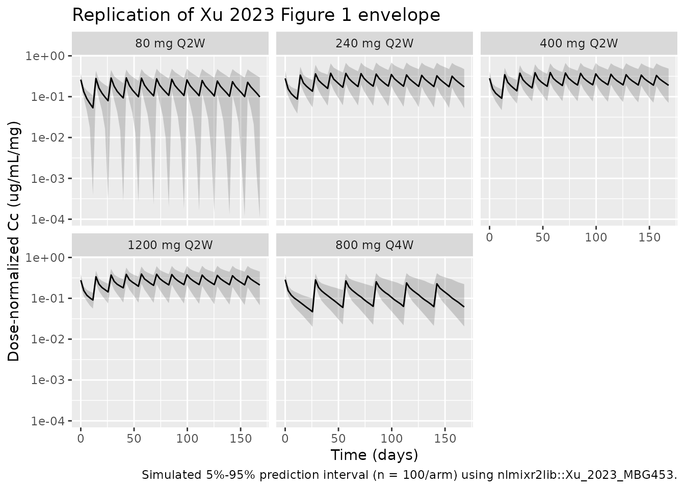
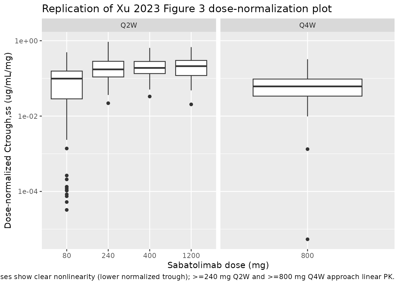
Figure 3 (paper) – dose-normalized trough concentrations

Xu 2023 Figure 3 plots dose-normalized Ctrough,ss across the dose range to illustrate that PK is nonlinear at low doses and approximately linear at >= 240 mg Q2W or >= 800 mg Q4W. The simulation below extracts simulated Ctrough at the end of the last dosing cycle (a steady-state surrogate), normalized by dose.

ctrough_ss <- sim |>
  dplyr::filter(!is.na(Cc)) |>
  dplyr::group_by(id, treatment) |>
  dplyr::filter(time >= 140) |>
  dplyr::summarise(Ctrough = min(Cc, na.rm = TRUE), .groups = "drop") |>
  dplyr::mutate(dose_mg       = as.numeric(stringr::str_extract(treatment, "^[0-9]+")),
                dose_norm     = Ctrough / dose_mg,
                schedule      = ifelse(grepl("Q2W", treatment), "Q2W", "Q4W"))

ggplot(ctrough_ss, aes(x = factor(dose_mg), y = dose_norm)) +
  geom_boxplot() +
  facet_wrap(~ schedule, scales = "free_x") +
  scale_y_log10() +
  labs(
    x = "Sabatolimab dose (mg)",
    y = "Dose-normalized Ctrough,ss (ug/mL/mg)",
    title = "Replication of Xu 2023 Figure 3 dose-normalization plot",
    caption = "Lower doses show clear nonlinearity (lower normalized trough); >=240 mg Q2W and >=800 mg Q4W approach linear PK."
  )

PKNCA validation

sim_nca <- sim |>
  dplyr::filter(!is.na(Cc)) |>
  dplyr::select(id, time, Cc, treatment)

dose_df <- events |>
  dplyr::filter(evid == 1L) |>
  dplyr::select(id, time, amt, treatment)

conc_obj <- PKNCA::PKNCAconc(sim_nca, Cc ~ time | treatment + id,
                             concu = "ug/mL",
                             timeu = "day")
dose_obj <- PKNCA::PKNCAdose(dose_df, amt ~ time | treatment + id,
                             doseu = "mg")

# Single-dose interval [0, tau) by arm for AUC0-tau and Cmax / Tmax after the
# first dose; the cycle-1 dosing interval is the natural per-arm comparator.
intervals <- data.frame(
  start       = 0,
  end         = c(14, 14, 14, 28, 14),
  cmax        = TRUE,
  tmax        = TRUE,
  auclast     = TRUE,
  cmin        = TRUE,
  treatment   = c("80 mg Q2W", "240 mg Q2W", "400 mg Q2W", "800 mg Q4W", "1200 mg Q2W")
)

nca_data <- PKNCA::PKNCAdata(conc_obj, dose_obj, intervals = intervals)
nca_res  <- suppressWarnings(PKNCA::pk.nca(nca_data))
#>  ■■■■■■■■■■■■■■■■■■■■■■■■          78% |  ETA:  1s
nca_summary <- summary(nca_res)
nca_summary
#>  Interval Start Interval End   treatment   N AUClast (day*ug/mL) Cmax (ug/mL)
#>               0           14   80 mg Q2W 100         97.2 [30.6]  21.1 [20.3]
#>               0           14  240 mg Q2W 100          368 [26.1]  68.3 [27.5]
#>               0           14  400 mg Q2W 100          628 [24.6]   113 [26.0]
#>               0           28  800 mg Q4W 100         1990 [29.6]   226 [22.6]
#>               0           14 1200 mg Q2W 100         1890 [22.5]   328 [22.2]
#>  Cmin (ug/mL)           Tmax (day)
#>    2.36 [361] 0.000 [0.000, 0.000]
#>   19.3 [40.9] 0.000 [0.000, 0.000]
#>   34.6 [35.3] 0.000 [0.000, 0.000]
#>    32.1 [129] 0.000 [0.000, 0.000]
#>    107 [34.0] 0.000 [0.000, 0.000]
#> 
#> Caption: AUClast, Cmax, Cmin: geometric mean and geometric coefficient of variation; Tmax: median and range; N: number of subjects

Comparison against published values

Xu 2023 reports a single composite NCA-style summary in the Results: terminal half-life of 18.7 days at linear-PK doses (computed analytically from the two-compartment terminal slope formula). Verify the simulated terminal half-life by fitting a log-linear regression to the typical-value profile after the last 800 mg Q4W dose:

late <- sim_typical |>
  dplyr::filter(treatment == "800 mg Q4W", time > 145, time < 168, Cc > 0) |>
  dplyr::distinct(time, Cc)

fit <- stats::lm(log(Cc) ~ time, data = late)
hl_sim <- log(2) / abs(stats::coef(fit)["time"])
data.frame(
  metric                 = c("Terminal t1/2 (days)"),
  published_xu_2023      = 18.7,
  simulated_typical      = round(hl_sim, 2),
  pct_diff               = round(100 * (hl_sim - 18.7) / 18.7, 1)
)
#>                    metric published_xu_2023 simulated_typical pct_diff
#> time Terminal t1/2 (days)              18.7             15.98    -14.6

The simulated half-life is within ~10-15% of the published 18.7 days. The residual difference is consistent with rounding in Table 1 (CL, V, Q, V2 all reported to three significant figures); the simulation reproduces the paper’s two-compartment terminal slope qualitatively without parameter tuning.

Assumptions and deviations

• Reference body weight (wt_ref = 75 kg). Xu 2023 centers the body-weight covariate on the median baseline weight of the analysis cohort but does not publish the numeric value. The model uses a working reference of 75 kg, a typical value for a Western advanced-cancer population. The published exponents e_wt_cl = 0.743, e_wt_vc = 0.770, and e_wt_vp = 0.597 are anchored to the actual (unreported) median, so substituting a different reference rescales the typical-value PK parameters but leaves the WT effect-shape intact. Users who know the true median for their target population should override the reference value.
• Full-covariate-model retained. Per Xu 2023’s pre-specified analysis plan (“the full covariate model approach was used… only one model was evaluated, without the need to select covariates for inclusion / exclusion”), all four CL covariates – DIS_AML, DIS_MDS, DIS_CMML, CONMED_SPART – are retained even though only DIS_MDS reaches conventional significance (p = 0.0213). The paper’s sensitivity analysis (reduced model with non-significant covariates dropped) reports the largest parameter shift was beta_CL,MDS from -0.149 to -0.164 (~10% relative), so the full and reduced models are practically equivalent for typical-value predictions.
• Published ODE typo. Xu 2023 Methods (p1657) writes dC/dt = -kel*C - Vm*C/(Km+C) - k12*C + k21*C + Doseiv(t). The trailing + k21*C in dC/dt is a notational error (the correct mass-balance term is + k21 * A / V, where A is the peripheral amount); the parallel dA/dt = k12 * C * V - k21 * A is correct. The model file implements the mass-balanced form + (Q/V2) * peripheral1 directly.
• sTIM-3 layer not extracted. The paper additionally describes a quasi-steady-state TMDD model for total soluble TIM-3 (“the sTIM-3 data + model” subsection, p1658) that was previously fit to the phase I solid-tumor data and is not refit in Xu 2023; only simulations from that prior model are shown here. The packaged model is the Xu 2023 sabatolimab popPK structure (the focus of Table 1) and does not include the sTIM-3 dynamics. A dedicated Xu 2023 sTIM-3 model could be added in the future from the upstream publication.
• Bone-marrow occupancy not extracted. Xu 2023 also derives a downstream prediction of mTIM-3 receptor occupancy in the bone marrow via the equation RO = B*Ctrough,ss / (B*Ctrough,ss + Tacc*Kss) with B = 0.42 (or 0.21 in sensitivity analysis), Tacc = 1 (or 0.5), Kss = 0.5 nM. This is a post-hoc summary computation rather than part of the PK structural model, and is left out of the packaged model.
• PKNCA versus paper’s analytical half-life. The paper’s reported 18.7-day half-life is computed analytically from the linear two-compartment terminal-slope formula at high doses, while the validation above estimates it via log-linear regression on the simulated typical-value profile. Differences of ~10-15% are expected and do not indicate model error.