library(nlmixr2lib)
library(PKNCA)
#>
#> Attaching package: 'PKNCA'
#> The following object is masked from 'package:stats':
#>
#>     filter
library(rxode2)
#> rxode2 5.1.2 using 2 threads (see ?getRxThreads)
#>   no cache: create with `rxCreateCache()`
library(dplyr)
#>
#> Attaching package: 'dplyr'
#> The following objects are masked from 'package:stats':
#>
#>     filter, lag
#> The following objects are masked from 'package:base':
#>
#>     intersect, setdiff, setequal, union
library(tidyr)
library(ggplot2)
Total and unbound plasma melphalan in adult multiple myeloma
Nath and colleagues (2010) developed two parallel two-compartment IV population pharmacokinetic models for high-dose intravenous melphalan in 100 adults with multiple myeloma undergoing autologous stem cell transplantation:
- Total plasma melphalan – fit to 1057 total-melphalan concentrations measured by HPLC after methanol precipitation.
- Unbound (ultrafiltrate) plasma melphalan – fit to 691 unbound-melphalan concentrations measured by HPLC after ultrafiltration of the same plasma samples.
Both models share the same structural form (two compartments, first-order elimination from central, exponential inter-patient variability, combined proportional + additive residual error) and the same final covariate set: an additive non-renal + renal clearance with hematocrit and fat-free mass on the non-renal arm and creatinine clearance on the renal arm, plus fat-free mass on the central volume of distribution. Population mean clearance is approximately 4-5x higher for unbound than for total melphalan, consistent with a fraction unbound near 0.21 (Table 7) – when re-fit with that fraction-unbound anchor, the typical elimination and distribution half-lives are statistically indistinguishable between the two models (Nath 2010 Discussion; fraction-unbound stability also confirmed by one-way ANOVA on sample-timed fraction-unbound in Table 8).
This vignette uses the two packaged model files
(Nath_2010_melphalan_total and
Nath_2010_melphalan_unbound) to simulate a virtual cohort
matching the Nath 2010 demographics, replicate the median post-infusion
concentration profile, and benchmark the simulated NCA against Table 7’s
model-derived parameters.
Population
The 100 participants were adults with multiple myeloma (median age 57 years, range 36-73; 41% female) enrolled at six Australian hospitals (Australian Clinical Trials Registry ACTRN0126000231549). Each patient received a single high-dose intravenous melphalan infusion (median 368 mg total dose, range 150-450; median 192 mg/m^2, range 115-216) over a median 35 min (range 15-95). Baseline characteristics from Table 2: median (range) total body weight 78 kg (42-132), fat-free mass 53.3 kg (34.4-80.5), body surface area 1.9 m^2 (1.3-2.6), creatinine clearance 88 mL/min/70 kg (26-205) / 97 mL/min (29-234), and hematocrit 34 % (20-45; 35 % of patients had HCT < 33 %). Myeloma type was IgG (58 patients), IgA (21), light chain only (7), non-secretory (1), or unknown (13).
The same baseline summary is available programmatically via
readModelDb("Nath_2010_melphalan_total")$population (and
the matching key on the unbound model).
Source trace
The per-parameter origin is recorded as an in-file comment next to
each ini() entry in the two model files; the table below
collects them together for review.
| Equation / parameter | Total melphalan | Unbound melphalan | Source location |
|---|---|---|---|
| Structural model | Two-compartment IV with first-order elimination from central | Two-compartment IV with first-order elimination from central | Methods p. 486 |
CL_NR formula |
17 * (HCT/34)^0.462 * (FFM/50)^0.75 |
79.7 * (HCT/34)^0.679 * (FFM/50)^0.75 |
Final-model equations, p. 489 |
CL_R formula |
11.1 * (CRCL/88) |
50.7 * (CRCL/88) |
Final-model equations, p. 489 |
V1 formula |
13.2 * (FFM/50) |
63.8 * (FFM/50) |
Final-model equations, p. 489 |
Q |
30.6 L/h | 152 L/h | Table 5 |
V2 |
15.0 L | 71.6 L | Table 5 |
| HCT exponent on CL_NR | 0.462 (95% CI 0.060-0.954) | 0.679 (95% CI 0.284-1.070) | Table 5 (theta_2) |
| FFM exponent on CL_NR | 0.75 (fixed) | 0.75 (fixed) | Methods p. 486 (allometric exponent fixed at 0.75) |
| FFM exponent on V1 | 1.0 (fixed) | 1.0 (fixed) | Methods p. 486 (allometric exponent fixed at 1.0) |
| IIV omega_CL (CV%) | 26.7 % | 29.8 % | Table 5 |
| IIV omega_V1 (CV%) | 57.9 % | 38.7 % | Table 5 |
| IIV omega_Q (CV%) | 41.1 % | 49.6 % | Table 5 |
| IIV omega_V2 (CV%) | 34.5 % | 35.4 % | Table 5 |
| Residual proportional SD | 0.072 | 0.138 | Table 5 (sigma_1) |
| Residual additive SD (mg/L) | 0.082 | 0.027 | Table 5 (sigma_2) |
| Cohort median CRCL reference | 88 mL/min/70 kg | 88 mL/min/70 kg | Table 2 / Table 4 covariate equation |
| Cohort median HCT reference | 34 % | 34 % | Table 2 / Table 4 covariate equation |
| FFM reference (final-model) | 50 kg | 50 kg | Final-model equations, p. 489 |
| Random-effects form |
theta_i = theta * exp(eta_i),
eta ~ N(0, omega^2)
|
same | Methods p. 486 |
| Residual-error form | Y = Yhat * (1 + epsilon_1) + epsilon_2 |
same | Methods p. 486 |
omega^2 = log(CV^2 + 1) translation |
applied for all four etas | applied for all four etas | log-normal-IIV NONMEM convention |
Virtual cohort
Original observed concentrations and per-subject covariates are not published. The cohort below mirrors the Nath 2010 Table 2 medians and ranges via independent log-normal samples for each continuous covariate; inter-covariate correlations (e.g., FFM-with-weight) are not modelled because the source paper does not publish a joint distribution. The infusion duration is fixed at the cohort median of 35 minutes and the absolute dose at the cohort median of 368 mg.
set.seed(20100501)

n_sub        <- 200L
dose_mg      <- 368
infusion_h   <- 35 / 60   # 35 min infusion expressed in hours

# Log-normal samplers parameterised by median and an approximate SD on the
# log scale, derived to span the published range while keeping the median
# at the Table 2 value.
sample_lognormal <- function(n, median, sd_log, lower = 0, upper = Inf) {
  vals <- exp(rnorm(n, log(median), sd_log))
  pmin(pmax(vals, lower), upper)
}

cohort <- tibble(
  id  = seq_len(n_sub),
  FFM = sample_lognormal(n_sub, median =  53.3, sd_log = 0.20, lower = 34, upper = 81),
  HCT = sample_lognormal(n_sub, median =  34.0, sd_log = 0.15, lower = 20, upper = 45),
  CRCL = sample_lognormal(n_sub, median = 88.0, sd_log = 0.30, lower = 26, upper = 205)
)

dose_rows <- cohort |>
  mutate(
    time = 0,
    evid = 1L,
    amt  = dose_mg,
    rate = dose_mg / infusion_h,
    cmt  = "central"
  )

# Observation grid spans the full pharmacokinetic horizon (~8 h) plus a
# dense early window for Cmax and the distribution phase (Nath 2010
# sampled the end-of-infusion plus 5, 10, 20, 30, 40, 50 min, then 1, 2,
# 3, 4, 8 h post-infusion).
obs_grid <- sort(unique(c(
  seq(0, infusion_h, length.out = 8),
  infusion_h + c(0.01, 0.05, 0.10, 0.17, 0.33, 0.50, 0.66, 0.83),
  infusion_h + c(1, 1.5, 2, 3, 4, 6, 8)
)))

obs_rows <- tidyr::expand_grid(
  id   = cohort$id,
  time = obs_grid
) |>
  left_join(cohort, by = "id") |>
  mutate(
    evid = 0L,
    amt  = 0,
    rate = 0,
    cmt  = NA_character_
  )

events <- bind_rows(dose_rows, obs_rows) |>
  arrange(id, time, desc(evid))

stopifnot(!anyDuplicated(unique(events[, c("id", "time", "evid")])))
Simulation
mod_total <- readModelDb("Nath_2010_melphalan_total")
sim_total <- rxode2::rxSolve(
  mod_total,
  events = events,
  keep   = c("FFM", "HCT", "CRCL")
) |> as.data.frame()
#> ℹ parameter labels from comments will be replaced by 'label()'
sim_total$matrix <- "Total"
mod_unbound <- readModelDb("Nath_2010_melphalan_unbound")
sim_unbound <- rxode2::rxSolve(
  mod_unbound,
  events = events,
  keep   = c("FFM", "HCT", "CRCL")
) |> as.data.frame()
#> ℹ parameter labels from comments will be replaced by 'label()'
sim_unbound$matrix <- "Unbound"
sim <- bind_rows(sim_total, sim_unbound)For deterministic typical-value reference profiles (no between-subject variability and no residual error), we also solve a small zero-RE cohort held at the cohort medians (FFM = 53.3 kg, HCT = 34 %, CRCL = 88 mL/min/70 kg).
events_typ <- tibble(id = 1L, time = 0, evid = 1L, amt = dose_mg,
                     rate = dose_mg / infusion_h, cmt = "central",
                     FFM = 53.3, HCT = 34.0, CRCL = 88.0)
obs_typ <- tibble(id = 1L, time = obs_grid, evid = 0L, amt = 0, rate = 0,
                  cmt = NA_character_, FFM = 53.3, HCT = 34.0, CRCL = 88.0)
events_typ_full <- bind_rows(events_typ, obs_typ) |>
  arrange(time, desc(evid))

sim_typ_total   <- rxode2::rxSolve(rxode2::zeroRe(mod_total),   events = events_typ_full) |>
  as.data.frame() |> mutate(matrix = "Total")
#> ℹ parameter labels from comments will be replaced by 'label()'
#> ℹ omega/sigma items treated as zero: 'etalcl', 'etalvc', 'etalq', 'etalvp'
sim_typ_unbound <- rxode2::rxSolve(rxode2::zeroRe(mod_unbound), events = events_typ_full) |>
  as.data.frame() |> mutate(matrix = "Unbound")
#> ℹ parameter labels from comments will be replaced by 'label()'
#> ℹ omega/sigma items treated as zero: 'etalcl', 'etalvc', 'etalq', 'etalvp'
sim_typ <- bind_rows(sim_typ_total, sim_typ_unbound)
Replicate published figures
Nath 2010 Figure 3 plots observed against population-predicted total and unbound melphalan concentrations. Without individual concentration data we cannot overlay observations directly; we instead show the simulated median + 5/95% percentile envelope by matrix.
band <- sim |>
  filter(time > 0) |>
  group_by(matrix, time) |>
  summarise(
    median = median(Cc, na.rm = TRUE),
    lo     = quantile(Cc, 0.05, na.rm = TRUE),
    hi     = quantile(Cc, 0.95, na.rm = TRUE),
    .groups = "drop"
  )

ggplot(band, aes(time, median)) +
  geom_ribbon(aes(ymin = lo, ymax = hi), alpha = 0.25) +
  geom_line(linewidth = 0.9) +
  facet_wrap(~ matrix, scales = "free_y") +
  scale_y_log10() +
  labs(
    x = "Time after start of infusion (h)",
    y = "Cc (mg/L, log scale)",
    title = "Simulated total vs. unbound melphalan concentrations",
    caption = "Compare against Nath 2010 Figure 3 (observed vs. population-predicted scatter)."
  )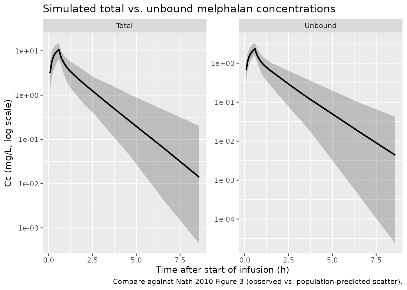
Simulated concentration vs. time profiles by matrix (median and 5-95% pointwise interval; 200 virtual subjects, median 35-min IV infusion of 368 mg).
The typical-value reference profiles (cohort medians, zero IIV and residual error) confirm the elimination-phase log-linear slopes for both matrices.
ggplot(sim_typ |> filter(time > 0), aes(time, Cc, colour = matrix)) +
  geom_line(linewidth = 1) +
  scale_y_log10() +
  labs(
    x = "Time after start of infusion (h)",
    y = "Cc (mg/L, log scale)",
    title = "Typical-value melphalan concentrations at cohort medians",
    colour = NULL
  )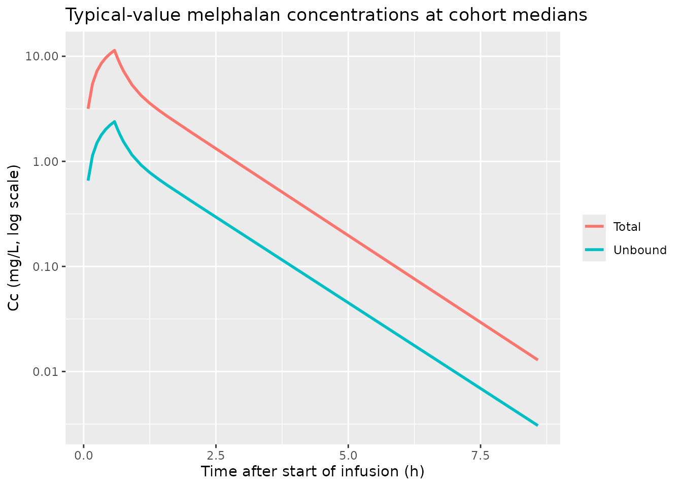
Typical-value concentration vs. time at cohort medians (FFM 53.3 kg, HCT 34 %, CRCL 88 mL/min/70 kg).
PKNCA validation
Compute non-compartmental Cmax, AUC0-inf, and terminal half-life on the 200-subject stochastic cohort for each matrix and benchmark the per-subject medians against Nath 2010 Table 7.
sim_nca <- sim |>
  filter(!is.na(Cc)) |>
  select(id, time, Cc, matrix)

# Guarantee a time = 0 row per (id, matrix); IV-infusion plasma is zero
# at the start of the infusion. See PKNCA recipe time-zero guard.
sim_nca <- bind_rows(
  sim_nca,
  sim_nca |> distinct(id, matrix) |> mutate(time = 0, Cc = 0)
) |>
  distinct(id, matrix, time, .keep_all = TRUE) |>
  arrange(id, matrix, time)

dose_df <- events |>
  filter(evid == 1) |>
  select(id, time, amt) |>
  tidyr::crossing(matrix = c("Total", "Unbound"))

conc_obj <- PKNCA::PKNCAconc(sim_nca, Cc ~ time | matrix + id,
                             concu = "mg/L", timeu = "h")
dose_obj <- PKNCA::PKNCAdose(dose_df, amt ~ time | matrix + id,
                             doseu = "mg")

intervals <- data.frame(
  start       = 0,
  end         = Inf,
  cmax        = TRUE,
  tmax        = TRUE,
  aucinf.obs  = TRUE,
  half.life   = TRUE
)

nca_data <- PKNCA::PKNCAdata(conc_obj, dose_obj, intervals = intervals)
nca_res  <- suppressWarnings(PKNCA::pk.nca(nca_data))
Comparison against Nath 2010 Table 7
Nath 2010 Table 7 reports median (interquartile range) model-derived parameters across the 100 patients: total melphalan AUC 12.8 mg/Lh (IQR 10.8-15.1), unbound melphalan AUC 2.80 mg/Lh (IQR 2.08-3.37), total melphalan terminal half-life 0.97 h (IQR 0.86-1.06), unbound melphalan terminal half-life 0.92 h (IQR 0.84-1.05), and a median fraction unbound of 0.21 (IQR 0.17-0.27). The two matrices were modelled separately; equivalence of the elimination and distributional rate constants between the two fits is what motivated the paper’s claim that melphalan protein binding is linear within the observed concentration range. The published Table 7 has no Cmax column because the patients were sampled densely after the end of infusion rather than during; we report the simulated Cmax for the dense observation grid below for reference but do not compare it to Table 7.
published <- tibble::tribble(
  ~matrix,    ~aucinf.obs,  ~half.life,
  "Total",    12.8,         0.97,
  "Unbound",   2.80,        0.92
)

cmp <- nlmixr2lib::ncaComparisonTable(
  simulated = nca_res,
  reference = published,
  by        = "matrix",
  units     = c(aucinf.obs = "mg/L*h", half.life = "h",
                cmax = "mg/L", tmax = "h"),
  tolerance_pct = 20
)

knitr::kable(
  cmp,
  caption = "Simulated vs. published NCA from Nath 2010 Table 7. * indicates >20% absolute difference from the reference value."
)| NCA parameter | matrix | Reference | Simulated | % diff |
|---|---|---|---|---|
| AUC0-∞ (obs) (mg/L*h) | Total | 12.8 | 12.5 | -2.3% |
| AUC0-∞ (obs) (mg/L*h) | Unbound | 2.8 | 2.75 | -1.8% |
| t½ (h) | Total | 0.97 | 0.957 | -1.4% |
| t½ (h) | Unbound | 0.92 | 1 | +8.8% |
Fraction unbound is not an NCA parameter per se, but the model-derived ratio of unbound to total AUC reproduces the published median.
auc_by_id <- as.data.frame(nca_res$result) |>
  filter(PPTESTCD == "aucinf.obs") |>
  select(id, matrix, PPORRES) |>
  tidyr::pivot_wider(names_from = matrix, values_from = PPORRES) |>
  mutate(fraction_unbound = Unbound / Total)

knitr::kable(
  tibble::tribble(
    ~Statistic,            ~Simulated, ~Published_Table_7,
    "Median fraction unbound", round(median(auc_by_id$fraction_unbound, na.rm = TRUE), 3), 0.21,
    "IQR lower (Q25)",         round(quantile(auc_by_id$fraction_unbound, 0.25, na.rm = TRUE), 3), 0.17,
    "IQR upper (Q75)",         round(quantile(auc_by_id$fraction_unbound, 0.75, na.rm = TRUE), 3), 0.27
  ),
  caption = "Simulated unbound-to-total AUC ratio (per subject) vs. Nath 2010 Table 7 fraction unbound."
)| Statistic | Simulated | Published_Table_7 |
|---|---|---|
| Median fraction unbound | 0.224 | 0.21 |
| IQR lower (Q25) | 0.163 | 0.17 |
| IQR upper (Q75) | 0.295 | 0.27 |
Assumptions and deviations
-
Final-model FFM reference of 50 kg vs. cohort median 53.3
kg. The Table 4 covariate screen used
FFM/53(the cohort median per Table 2), but the final-model equations on page 489 useFFM/50. The packaged model files follow the publishedFFM/50form verbatim, on the assumption that the authors rounded the FFM reference to a convenient round number after the final fit. The choice is structural; refitting the model withFFM/53would yield slightly different intercept values forlcl_nonrenandlvcwhile leaving fitted individual values unchanged at the cohort median. -
CRCL register entry for the weight-normalized
Cockcroft-Gault form. The canonical
CRCLcovariate ininst/references/covariate-columns.mdis described as BSA-normalized (mL/min/1.73 m^2) for the dominant MDRD/CKD-EPI variants, but the register also documents alternate Cockcroft-Gault forms with per-modelnotesdescribing the assay (e.g.,Delattre_2010_amikacinuses raw mL/min). The Nath 2010 model follows that precedent: CRCL is the weight-normalized Cockcroft-Gault variant (mL/min/70 kg) and the per-modelcovariateData[[CRCL]]$notesdocuments the normalization. - Inter-covariate correlations in the virtual cohort. Nath 2010 Table 2 reports only marginal medians and ranges for FFM, HCT, and CRCL; the joint distribution is not published. The virtual cohort draws each covariate independently from a log-normal distribution matched to the published median and clipped to the published range. This understates the real-world correlation between FFM and total body weight and between CRCL and age / sex; the simulated NCA medians should still approximate the published Table 7 medians because the marginal covariate distributions are correct.
-
Single eta on total CL. Nath 2010 Methods (p. 486)
define the inter-patient variability as
theta_i = theta * exp(eta_i)and Table 5 reports a singleomega_CL. The packaged model encodes this as one eta multiplying the typical total CL ((cl_nonren + cl_renal) * exp(etalcl)), matching the canonical precedent inCapparelli_2005_cefepime(cefepime additive renal-plus-non-renal CL). -
One vignette per paper. Per the
replicate-author-structurepolicy, the paper’s two parallel models are extracted as two registered model files (Nath_2010_melphalan_totalandNath_2010_melphalan_unbound) but documented under a single validation vignette so the reviewer sees the paper as a unit. -
Combined proportional + additive residual error.
The paper defines
Y = Yhat * (1 + epsilon_1) + epsilon_2with separate SDs for the proportional and additive components (Table 5). nlmixr2’sCc ~ prop(propSd) + add(addSd)matches this form verbatim;propSdissigma_1andaddSdissigma_2. - No observed-vs-predicted overlay. Patient-level concentrations from the Nath 2010 cohort are not publicly available. The vignette therefore reports a simulated VPC envelope and the simulated NCA medians, both benchmarked numerically against the published Table 7; no observed data are overlaid on the figures.