Tacrolimus in pediatric HSCT (Liu 2022) • nlmixr2lib

Model and source

Citation: Liu XL, Guan YP, Wang Y, Huang K, Jiang FL, Wang J, Yu QH, Qiu KF, Huang M, Wu JY, Zhou DH, Zhong GP, Yu XX. Population Pharmacokinetics and Initial Dosage Optimization of Tacrolimus in Pediatric Hematopoietic Stem Cell Transplant Patients. Front Pharmacol. 2022;13:891648. doi:10.3389/fphar.2022.891648
Description (model 1): One-compartment population pharmacokinetic model for intravenous (continuous 24 h infusion) and oral tacrolimus in pediatric hematopoietic stem cell transplant (HSCT) recipients (Liu 2022, final model 1, n = 86): first-order absorption with ka fixed at 4.48 1/h and an estimated oral bioavailability; power effects of body weight and hematocrit on CL, exponential effects of concomitant azole antifungals, concomitant caspofungin and post-transplant day >= 28 on CL, and a power effect of hematocrit on V.
Description (model 2): One-compartment population pharmacokinetic model for intravenous (continuous 24 h infusion) and oral tacrolimus in the CYP3A5-genotyped subpopulation of pediatric hematopoietic stem cell transplant (HSCT) recipients (Liu 2022, model 2, n = 24): the model 1 structure re-estimated with an added exponential CYP3A5 expresser (*1 carrier) effect on CL; ka fixed at 4.48 1/h with an estimated oral bioavailability.
Article: https://doi.org/10.3389/fphar.2022.891648 (open access)

Liu 2022 developed two population PK models from routine tacrolimus trough monitoring in children after allogeneic hematopoietic stem cell transplantation (HSCT):

Model 1 (Liu_2022_tacrolimus) – the final model fitted to all 86 patients.
Model 2 (Liu_2022_tacrolimus_cyp3a5) – the model 1 structure re-estimated in the 24 patients with a CYP3A5 genotype, with an added CYP3A5 expresser effect on clearance.

Both are one-compartment models with first-order absorption (ka fixed at 4.48 1/h because only troughs were sampled), an estimated oral bioavailability F, and IV doses given as a continuous 24 h infusion.

Population

Liu 2022 Table 1: 86 children (53 boys, 33 girls), median age 5 years (range 1-16), median weight 17.4 kg (6.0-50.0), treated at Sun Yat-sen Memorial Hospital, Guangzhou, China, between January 2017 and December 2020. Diagnoses were beta-thalassemia (27.9%), acute lymphatic leukemia (25.6%), acute myelogenous leukemia (19.8%), aplastic anemia (11.6%) and others; 80.2% had unrelated donors and 70.9% developed acute GVHD. The 578 whole-blood trough concentrations (EMIT assay) were split 320 IV and 258 oral; median doses were 0.024 mg/kg/day IV and 0.057 mg/kg/day oral. Laboratory values (Table 2) include a median hematocrit of 0.289 (0.166-0.445) and hemoglobin 96.5 g/L (54-150). The CYP3A5 subpopulation (model 2) comprised 24 patients: one *1/*1, and about half each *1/*3 and *3/*3.

The same information is available programmatically via readModelDb("Liu_2022_tacrolimus")()$population.

Source trace

Every ini() value carries an in-file comment pointing to its source. The covariate equations are Liu 2022 Eqs. 4-5 (model 1) and Eqs. 6-7 (model 2).

Parameter	Model 1	Model 2	Source location
`lka` (ka, 1/h)	fixed(log(4.48))	fixed(log(4.48))	Table 3; Results (‘fixed at 4.48 according to the literature’)
`lcl` (CL, L/h)	log(2.42)	log(2.41)	Table 3; Eqs. 4 / 6
`lvc` (V, L)	log(79.6)	log(92.9)	Table 3; Eqs. 5 / 7
`lfdepot` (F)	log(0.19)	log(0.25)	Table 3
`e_wt_cl`	0.56	0.48	Table 3 theta WT,CL; Eqs. 4 / 6 (WT / 17.8)
`e_hct_cl`	-0.66	-1.06	Table 3 theta Hct,CL; Eqs. 4 / 6 (Hct / 0.296)
`e_conmed_azole_cl`	-0.40	-0.39	Table 3 theta CZ,CL; exponential
`e_conmed_caspofungin_cl`	0.16	0.04	Table 3 theta CPFG,CL; exponential
`e_pod_cl`	-0.32	-0.33	Table 3 theta PTD,CL; applied when PTD = 2 (day >= 28)
`e_cyp3a5_expr_cl`	–	0.32	Table 3 theta CYP3A53,CL; Eq. 6 ‘if CYP3A51 carriers’
`e_hct_vc`	-0.66	-0.60	Table 3 theta Hct,V; Eqs. 5 / 7 (Hct / 0.289)
`etalcl` (omega^2)	0.06	0.02	Table 3
`etalvc` (omega^2)	0.66	0.66	Table 3
`etalfdepot` (omega^2)	0.51	0.25	Table 3
`propSd`	0.374	0.368	Table 3 sigma proportional (%)
IIV form `P * exp(eta)`	–	–	Methods Eq. 1
`Cc = 1000 * central / vc`	–	–	mg / L to ng/mL

Model 1: typical-patient simulations (Table 4)

Liu 2022 Table 4 gives the median and 10th-90th percentiles of the simulated trough concentration (C0) for a “typical patient” (17.4 kg, hemoglobin 97 g/L) under three IV doses (continuous 24 h infusion) and three oral doses (q12h). Hematocrit is derived from hemoglobin with the paper’s regression HCT = 0.0029 * Hgb + 0.0038 (Discussion), giving 28.5%. The paper does not state the post-transplant day, the comedications or the day the trough was taken; this vignette uses post-transplant day 40 (PTD = 2), no azole or caspofungin, and the trough at the end of day 14 (see the Assumptions section for why).

hgb_to_hct <- function(hgb) 100 * (0.0029 * hgb + 0.0038)

regimens <- tibble::tribble(
  ~treatment,           ~route, ~dose_mgkgday,
  "IV 0.01 mg/kg/day",  "iv",   0.01,
  "IV 0.025 mg/kg/day", "iv",   0.025,
  "IV 0.05 mg/kg/day",  "iv",   0.05,
  "PO 0.05 mg/kg/day",  "oral", 0.05,
  "PO 0.1 mg/kg/day",   "oral", 0.1,
  "PO 0.2 mg/kg/day",   "oral", 0.2
)

# One subject's events for a regimen: 14 days of dosing, dense sampling over
# the last dosing interval so PKNCA sees the full steady-state profile, plus
# the day-7 trough.
make_subject_events <- function(id, route, dose_mgkgday, wt, hgb, pod,
                                azole = 0, caspo = 0, cyp = NULL) {
  daily <- dose_mgkgday * wt
  if (route == "iv") {
    doses <- data.frame(
      time = seq(0, 312, by = 24), amt = daily, rate = daily / 24,
      cmt = "central", evid = 1L
    )
    obs_t <- c(168, seq(312, 336, by = 2))
  } else {
    doses <- data.frame(
      time = seq(0, 324, by = 12), amt = daily / 2, rate = 0,
      cmt = "depot", evid = 1L
    )
    obs_t <- c(168, seq(324, 336, by = 1))
  }
  obs <- data.frame(time = obs_t, amt = 0, rate = 0, cmt = "central", evid = 0L)
  out <- dplyr::bind_rows(doses, obs) |>
    dplyr::arrange(time, dplyr::desc(evid)) |>
    dplyr::mutate(
      id = id, WT = wt, HCT = hgb_to_hct(hgb), POD = pod,
      CONMED_AZOLE = azole, CONMED_CASPOFUNGIN = caspo
    )
  if (!is.null(cyp)) out$CYP3A5_EXPR <- cyp
  out
}

n_per_arm <- 200L
events_t4 <- dplyr::bind_rows(lapply(seq_len(nrow(regimens)), function(i) {
  ids <- (i - 1L) * n_per_arm + seq_len(n_per_arm)
  dplyr::bind_rows(lapply(ids, make_subject_events,
    route = regimens$route[i], dose_mgkgday = regimens$dose_mgkgday[i],
    wt = 17.4, hgb = 97, pod = 40
  )) |>
    dplyr::mutate(treatment = regimens$treatment[i])
}))
stopifnot(!anyDuplicated(unique(events_t4[, c("id", "time", "evid")])))

mod1 <- readModelDb("Liu_2022_tacrolimus")
rxode2::rxSetSeed(20220706)
sim_t4 <- rxode2::rxSolve(mod1, events = events_t4, keep = "treatment") |>
  as.data.frame()
#> ℹ parameter labels from comments will be replaced by 'label()'

PKNCA over the day-14 dosing interval

sim_nca <- sim_t4 |>
  dplyr::filter(!is.na(Cc)) |>
  dplyr::select(id, time, Cc, treatment)
sim_nca <- dplyr::bind_rows(
  sim_nca,
  sim_nca |> dplyr::distinct(id, treatment) |> dplyr::mutate(time = 0, Cc = 0)
) |>
  dplyr::distinct(id, treatment, time, .keep_all = TRUE) |>
  dplyr::arrange(id, treatment, time)

dose_df <- events_t4 |>
  dplyr::filter(evid == 1) |>
  dplyr::select(id, time, amt, treatment)

conc_obj <- PKNCA::PKNCAconc(sim_nca, Cc ~ time | treatment + id)
dose_obj <- PKNCA::PKNCAdose(dose_df, amt ~ time | treatment + id)

intervals <- regimens |>
  dplyr::transmute(
    treatment,
    start = ifelse(route == "iv", 312, 324),
    end = 336,
    cmin = TRUE, cmax = TRUE, cav = TRUE
  ) |>
  as.data.frame()

nca_res <- PKNCA::pk.nca(PKNCA::PKNCAdata(conc_obj, dose_obj, intervals = intervals))

published_t4 <- data.frame(
  treatment = regimens$treatment,
  cmin = c(3.6, 9.2, 18.3, 3.0, 6.1, 13.2)
)
cmp_t4 <- nlmixr2lib::ncaComparisonTable(
  simulated = nca_res,
  reference = published_t4,
  by = "treatment",
  params = "cmin",
  units = c(cmin = "ng/mL"),
  tolerance_pct = 20
)
knitr::kable(
  cmp_t4,
  caption = paste(
    "Median trough (Cmin over the day-14 dosing interval) vs. Liu 2022",
    "Table 4 medians. * differs from the reference by >20%."
  )
)

Median trough (Cmin over the day-14 dosing interval) vs. Liu 2022 Table 4 medians. * differs from the reference by >20%.
NCA parameter	treatment	Reference	Simulated	% diff
Cmin (ng/mL)	IV 0.01 mg/kg/day	3.6	4.02	+11.8%
Cmin (ng/mL)	IV 0.025 mg/kg/day	9.2	9.76	+6.0%
Cmin (ng/mL)	IV 0.05 mg/kg/day	18.3	19.8	+8.2%
Cmin (ng/mL)	PO 0.05 mg/kg/day	3	3.01	+0.2%
Cmin (ng/mL)	PO 0.1 mg/kg/day	6.1	6.27	+2.8%
Cmin (ng/mL)	PO 0.2 mg/kg/day	13.2	11.8	-10.5%

The published 10th-90th percentile ranges are compared below with the simulated ranges, with (sim) and without (Cc) residual error, at both the day-7 and the day-14 trough.

published_pct <- tibble::tribble(
  ~treatment,           ~published,
  "IV 0.01 mg/kg/day",  "3.6 (2.1-6.4)",
  "IV 0.025 mg/kg/day", "9.2 (5.2-16.3)",
  "IV 0.05 mg/kg/day",  "18.3 (10.6-31.2)",
  "PO 0.05 mg/kg/day",  "3.0 (1.0-8.4)",
  "PO 0.1 mg/kg/day",   "6.1 (1.9-17.8)",
  "PO 0.2 mg/kg/day",   "13.2 (4.1-36.1)"
)
fmt_q <- function(x) {
  q <- stats::quantile(x, c(0.5, 0.1, 0.9))
  sprintf("%.1f (%.1f-%.1f)", q[1], q[2], q[3])
}
trough_tab <- sim_t4 |>
  dplyr::filter(time %in% c(168, 336)) |>
  dplyr::group_by(treatment, time) |>
  dplyr::summarise(ipred = fmt_q(Cc), with_ruv = fmt_q(sim), .groups = "drop") |>
  tidyr::pivot_wider(names_from = time, values_from = c(ipred, with_ruv)) |>
  dplyr::left_join(published_pct, by = "treatment") |>
  dplyr::mutate(treatment = factor(treatment, levels = regimens$treatment)) |>
  dplyr::arrange(treatment)
trough_tab |>
  dplyr::select(
    treatment, published, ipred_168, with_ruv_168, ipred_336, with_ruv_336
  ) |>
  dplyr::rename(
    "Regimen" = treatment,
    "Liu 2022 Table 4" = published,
    "Day 7, no RUV" = ipred_168,
    "Day 7, with RUV" = with_ruv_168,
    "Day 14, no RUV" = ipred_336,
    "Day 14, with RUV" = with_ruv_336
  ) |>
  knitr::kable(caption = "Trough C0 (ng/mL), median (10th-90th percentile).")

Trough C0 (ng/mL), median (10th-90th percentile).
Regimen	Liu 2022 Table 4	Day 7, no RUV	Day 7, with RUV	Day 14, no RUV	Day 14, with RUV
IV 0.01 mg/kg/day	3.6 (2.1-6.4)	3.8 (2.6-5.0)	3.4 (1.5-5.7)	4.0 (2.8-5.4)	3.8 (1.8-6.4)
IV 0.025 mg/kg/day	9.2 (5.2-16.3)	9.0 (6.7-12.4)	8.7 (4.2-14.0)	9.8 (7.5-13.0)	9.4 (4.1-15.6)
IV 0.05 mg/kg/day	18.3 (10.6-31.2)	18.5 (13.4-24.9)	17.5 (8.6-29.6)	19.8 (14.7-26.4)	18.9 (10.4-32.1)
PO 0.05 mg/kg/day	3.0 (1.0-8.4)	2.9 (0.9-7.1)	2.7 (0.8-7.1)	3.0 (1.0-7.9)	2.9 (0.8-8.9)
PO 0.1 mg/kg/day	6.1 (1.9-17.8)	5.7 (2.0-15.9)	5.1 (1.8-17.0)	6.3 (2.2-17.8)	5.8 (1.7-18.8)
PO 0.2 mg/kg/day	13.2 (4.1-36.1)	10.2 (4.2-28.9)	10.1 (3.5-33.2)	11.8 (4.7-32.0)	10.8 (3.4-33.4)

pct_diff_t4 <- sim_t4 |>
  dplyr::filter(time == 336) |>
  dplyr::group_by(treatment) |>
  dplyr::summarise(med = stats::median(Cc), .groups = "drop") |>
  dplyr::inner_join(published_t4, by = "treatment") |>
  dplyr::mutate(pct_diff = 100 * (med - cmin) / cmin)
pct_diff_t4
#> # A tibble: 6 × 4
#>   treatment            med  cmin pct_diff
#>   <chr>              <dbl> <dbl>    <dbl>
#> 1 IV 0.01 mg/kg/day   4.04   3.6   12.3  
#> 2 IV 0.025 mg/kg/day  9.79   9.2    6.41 
#> 3 IV 0.05 mg/kg/day  19.8   18.3    8.26 
#> 4 PO 0.05 mg/kg/day   3.01   3      0.371
#> 5 PO 0.1 mg/kg/day    6.27   6.1    2.77 
#> 6 PO 0.2 mg/kg/day   11.8   13.2  -10.4
stopifnot(
  # Structural: a mis-transcribed CL, F, covariate centring or unit would
  # shift every regimen by tens of percent. The day-14 medians observed
  # while authoring ranged from -10% (PO 0.2) to +12% (IV 0.01) of the
  # published values, with a median of about +4%.
  abs(stats::median(pct_diff_t4$pct_diff)) < 15,
  # Envelope across regimens; robust to which subjects land in the tails.
  stats::quantile(abs(pct_diff_t4$pct_diff), 0.9) < 25
)

The IV troughs scale linearly with dose, as they must for a linear model, and the medians match Table 4 to within about 12%. The simulated IV medians run 6-12% above the published ones at day 14. The oral medians scatter on both sides of the published values, as expected for a 200-subject median with the large IIV on F.

Closed-form check of the IV steady state

For a continuous infusion at rate k0, the steady-state concentration is k0 / CL, independent of V and F. The typical-value solve after 30 days (more than 20 half-lives) must reproduce it.

ev_ss <- make_subject_events(1L, "iv", 0.025, wt = 17.4, hgb = 97, pod = 40)
ev_ss <- dplyr::bind_rows(
  ev_ss |> dplyr::filter(evid == 1) |>
    dplyr::select(-time) |>
    dplyr::slice(1) |>
    tidyr::crossing(time = seq(0, 696, by = 24)),
  ev_ss |> dplyr::filter(evid == 0) |> dplyr::slice(1) |> dplyr::mutate(time = 720)
) |>
  dplyr::arrange(time, dplyr::desc(evid))
sim_ss <- rxode2::rxSolve(rxode2::zeroRe(mod1), events = ev_ss) |> as.data.frame()
#> ℹ parameter labels from comments will be replaced by 'label()'
#> ℹ omega/sigma items treated as zero: 'etalcl', 'etalvc', 'etalfdepot'
cl_typ <- 2.42 * (17.4 / 17.8)^0.56 * (hgb_to_hct(97) / 29.6)^-0.66 * exp(-0.32)
css_closed <- 1000 * (0.025 * 17.4 / 24) / cl_typ
c(simulated = sim_ss$Cc[sim_ss$time == 720], closed_form = css_closed)
#>   simulated closed_form 
#>    10.19084    10.19084
stopifnot(abs(sim_ss$Cc[sim_ss$time == 720] / css_closed - 1) < 1e-4)

Model 1: hemoglobin and azole effects (Figure 3)

Figure 3 of Liu 2022 shows simulated trough concentrations of the typical patient at hemoglobin 70, 90, 110 and 130 g/L, with and without azole antifungals, for the IV and oral regimens. The box plots below replicate it (day-14 trough, PTD = 2, 100 virtual patients per box; whiskers 5th-95th percentiles).

fig3_grid <- tidyr::crossing(
  regimens,
  hgb = c(70, 90, 110, 130),
  azole = c(0, 1)
)
n_fig3 <- 100L
events_f3 <- dplyr::bind_rows(lapply(seq_len(nrow(fig3_grid)), function(i) {
  ids <- (i - 1L) * n_fig3 + seq_len(n_fig3)
  dplyr::bind_rows(lapply(ids, make_subject_events,
    route = fig3_grid$route[i], dose_mgkgday = fig3_grid$dose_mgkgday[i],
    wt = 17.4, hgb = fig3_grid$hgb[i], pod = 40, azole = fig3_grid$azole[i]
  )) |>
    dplyr::filter(evid == 1 | time == 336) |>
    dplyr::mutate(
      treatment = fig3_grid$treatment[i], hgb = fig3_grid$hgb[i],
      azole = fig3_grid$azole[i]
    )
}))
stopifnot(!anyDuplicated(unique(events_f3[, c("id", "time", "evid")])))
sim_f3 <- rxode2::rxSolve(mod1, events = events_f3,
                          keep = c("treatment", "hgb", "azole")) |>
  as.data.frame() |>
  dplyr::mutate(
    route = ifelse(grepl("^IV", treatment), "IV", "Oral (q12h)"),
    azole_lab = ifelse(azole == 1, "with azole", "without azole"),
    treatment = factor(treatment, levels = regimens$treatment)
  )

sim_f3 |>
  dplyr::group_by(route, azole_lab, treatment, hgb) |>
  dplyr::summarise(
    q05 = stats::quantile(Cc, 0.05), q25 = stats::quantile(Cc, 0.25),
    q50 = stats::median(Cc), q75 = stats::quantile(Cc, 0.75),
    q95 = stats::quantile(Cc, 0.95), .groups = "drop"
  ) |>
  ggplot(aes(x = factor(hgb), colour = treatment)) +
  annotate("rect", xmin = -Inf, xmax = Inf, ymin = 5, ymax = 15,
           alpha = 0.15, fill = "grey40") +
  geom_boxplot(
    aes(ymin = q05, lower = q25, middle = q50, upper = q75, ymax = q95),
    stat = "identity", position = position_dodge(width = 0.8), width = 0.7
  ) +
  facet_grid(route ~ azole_lab) +
  labs(
    x = "Hemoglobin (g/L)", y = "Tacrolimus trough (ng/mL)", colour = NULL,
    caption = "Replicates Figure 3 of Liu 2022 (shaded band: 5-15 ng/mL)."
  ) +
  theme_bw() +
  theme(legend.position = "bottom")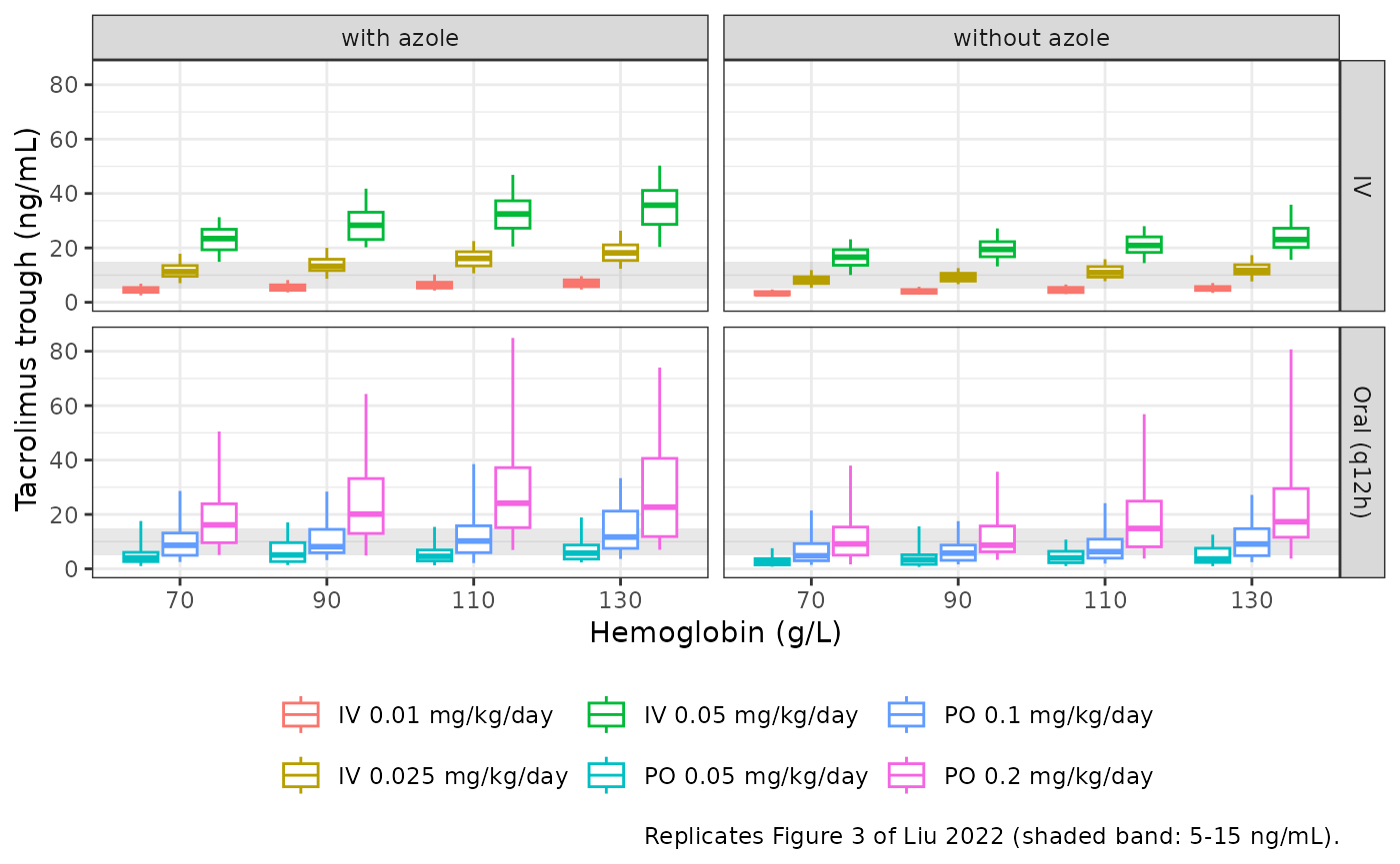

sim_f3 |>
  dplyr::filter(treatment == "IV 0.05 mg/kg/day", azole == 0) |>
  dplyr::group_by(hgb) |>
  dplyr::summarise(median_C0 = stats::median(Cc), .groups = "drop") |>
  dplyr::rename("Hemoglobin (g/L)" = hgb, "Median C0 (ng/mL)" = median_C0) |>
  knitr::kable(digits = 1, caption = "IV 0.05 mg/kg/day without azole.")

IV 0.05 mg/kg/day without azole.
Hemoglobin (g/L)	Median C0 (ng/mL)
70	16.6
90	19.4
110	20.9
130	23.1

Higher hemoglobin (hematocrit) lowers clearance and so raises the trough, and azole comedication raises it by exp(0.40) = 1.49-fold, as in Figure 3. Read by eye from Figure 3A, the published medians at 0.05 mg/kg/day IV are about 13.7, 17, 21 and 22.6 ng/mL at 70, 90, 110 and 130 g/L. The simulation (table above) agrees to within about 15% from 90 to 130 g/L. At 70 g/L it is about 20% higher than the figure. The figure implies a steeper hemoglobin dependence (130 vs 70 g/L ratio about 1.65) than Eq. 4 gives at steady state ((38.1 / 20.7)^0.66 = 1.50). Because CL and V carry the same hematocrit exponent, their ratio and so the time to steady state do not depend on hematocrit, so an earlier trough day would not explain the difference. It is recorded as a known deviation below.

Model 2: CYP3A5 genotype dosing tables (Supplementary Tables S3 and S4)

Supplementary Tables S3 (IV) and S4 (oral) of Liu 2022 list the model-2-recommended daily doses by post-transplant period, CYP3A5 genotype, azole use and weight that reach a trough target of 5 or 10 ng/mL. The criterion used to pick the dose is not stated. The check below simulates the typical trough on day 14 at each recommended dose (hemoglobin 97 g/L, PTD 1 taken as day 14, PTD 2 as day 40) and compares it with the target.

s34 <- tidyr::crossing(
  pod = c(14, 40),
  grp = 1:4,
  WT = c(10, 20, 30, 40, 50)
) |>
  dplyr::mutate(
    CYP3A5_EXPR = ifelse(grp <= 2, 1, 0),
    CONMED_AZOLE = ifelse(grp %in% c(2, 4), 1, 0)
  )
# Column order follows the supplementary tables: PTD <= 1 month then
# > 1 month; within each, *1 carrier without azole, *1 carrier with azole,
# *3/*3 without azole, *3/*3 with azole; weights 10-50 kg.
s34$iv_5 <- c(
  .05, .05, .025, .025, .025, .05, .025, .025, .015, .015,
  .05, .025, .025, .025, .015, .025, .025, .015, .01, .01,
  .05, .025, .025, .025, .015, .025, .025, .015, .01, .01,
  .05, .025, .025, .015, .01, .025, .025, .01, .01, .01
)
s34$iv_10 <- c(
  .06, .06, .05, .035, .035, .06, .05, .035, .025, .025,
  .06, .05, .035, .035, .025, .05, .035, .025, .025, .015,
  .06, .05, .03, .035, .025, .05, .035, .025, .025, .015,
  .06, .05, .035, .025, .025, .05, .035, .025, .015, .015
)
s34$oral_5 <- c(
  .2, .15, .1, .1, .1, .15, .1, .1, .05, .05,
  .15, .1, .1, .1, .05, .1, .1, .05, .05, .05,
  .2, .1, .1, .1, .1, .1, .1, .05, .05, .05,
  .15, .1, .1, .05, .05, .1, .05, .05, .05, .05
)
s34$oral_10 <- c(
  .25, .2, .2, .2, .15, .2, .15, .15, .1, .1,
  .2, .2, .15, .15, .15, .2, .15, .1, .1, .1,
  .25, .2, .15, .15, .15, .2, .15, .1, .1, .1,
  .2, .15, .15, .1, .1, .2, .1, .1, .07, .07
)
s34_long <- s34 |>
  tidyr::pivot_longer(c(iv_5, iv_10, oral_5, oral_10),
                      names_to = c("route", "target"), names_sep = "_",
                      values_to = "dose_mgkgday") |>
  dplyr::mutate(target = as.numeric(target), id = dplyr::row_number())

events_s34 <- dplyr::bind_rows(lapply(seq_len(nrow(s34_long)), function(i) {
  r <- s34_long[i, ]
  make_subject_events(r$id, r$route, r$dose_mgkgday, wt = r$WT, hgb = 97,
                      pod = r$pod, azole = r$CONMED_AZOLE, cyp = r$CYP3A5_EXPR) |>
    dplyr::filter(evid == 1 | time == 336)
}))
mod2 <- readModelDb("Liu_2022_tacrolimus_cyp3a5")
sim_s34 <- rxode2::rxSolve(rxode2::zeroRe(mod2), events = events_s34) |>
  as.data.frame() |>
  dplyr::select(id, Cc)
#> ℹ parameter labels from comments will be replaced by 'label()'
#> ℹ omega/sigma items treated as zero: 'etalcl', 'etalvc', 'etalfdepot'
#> Warning: multi-subject simulation without without 'omega'
res_s34 <- s34_long |>
  dplyr::inner_join(sim_s34, by = "id") |>
  dplyr::mutate(ratio = Cc / target)

res_s34 |>
  dplyr::mutate(
    period = ifelse(pod == 14, "PTD <= 1 month", "PTD > 1 month"),
    genotype = ifelse(CYP3A5_EXPR == 1, "expresser (*1 carrier)", "non-expresser")
  ) |>
  dplyr::group_by(route, target, period, genotype) |>
  dplyr::summarise(
    median_ratio = stats::median(ratio),
    range_ratio = sprintf("%.2f-%.2f", min(ratio), max(ratio)),
    .groups = "drop"
  ) |>
  dplyr::rename(
    "Route" = route, "Target (ng/mL)" = target, "Period" = period,
    "CYP3A5" = genotype,
    "Median typical C0 / target" = median_ratio,
    "Range over weight and azole" = range_ratio
  ) |>
  knitr::kable(digits = 2, caption = paste(
    "Typical day-14 trough at the Liu 2022 recommended doses divided by",
    "the target trough."
  ))

Typical day-14 trough at the Liu 2022 recommended doses divided by the target trough.
Route	Target (ng/mL)	Period	CYP3A5	Median typical C0 / target	Range over weight and azole
iv	5	PTD <= 1 month	expresser (*1 carrier)	1.66	1.41-2.35
iv	5	PTD <= 1 month	non-expresser	1.66	1.33-2.32
iv	5	PTD > 1 month	expresser (*1 carrier)	1.68	1.34-2.34
iv	5	PTD > 1 month	non-expresser	2.12	1.41-3.20
iv	10	PTD <= 1 month	expresser (*1 carrier)	1.36	0.95-1.68
iv	10	PTD <= 1 month	non-expresser	1.50	1.12-1.66
iv	10	PTD > 1 month	expresser (*1 carrier)	1.52	1.13-1.68
iv	10	PTD > 1 month	non-expresser	1.85	1.39-2.24
oral	5	PTD <= 1 month	expresser (*1 carrier)	1.31	0.97-1.72
oral	5	PTD <= 1 month	non-expresser	1.47	0.97-2.07
oral	5	PTD > 1 month	expresser (*1 carrier)	1.59	1.26-2.09
oral	5	PTD > 1 month	non-expresser	1.99	1.32-2.33
oral	10	PTD <= 1 month	expresser (*1 carrier)	1.05	0.84-1.29
oral	10	PTD <= 1 month	non-expresser	1.38	0.97-1.56
oral	10	PTD > 1 month	expresser (*1 carrier)	1.39	1.20-1.58
oral	10	PTD > 1 month	non-expresser	1.47	1.32-2.05


summary(res_s34$ratio)
#>    Min. 1st Qu.  Median    Mean 3rd Qu.    Max. 
#>  0.8422  1.3321  1.5139  1.5854  1.7823  3.1963

stopifnot(
  # Deterministic (typical-value) solve. At the recommended doses the
  # typical trough reaches the target (ratios observed while authoring
  # 0.84-3.20, median about 1.5): the doses are rounded to a coarse grid
  # (0.01, 0.015, 0.025, 0.035, 0.05 ... mg/kg/day), whose steps are up to
  # 2-fold.
  stats::median(res_s34$ratio) > 1,
  stats::median(res_s34$ratio) < 2,
  min(res_s34$ratio) > 0.75
)

The recommended doses deliver the target trough or somewhat more in the typical patient. Because doses are rounded to a coarse grid, the typical trough sits about 1.5-fold above target on average. The published tables also recommend the same or higher doses for *3/*3 non-expressers than for *1 carriers in several cells, which is the opposite of what model 2 implies (non-expressers have 27% lower CL). This suggests the tables come from a stochastic criterion and coarse rounding rather than from the typical value alone.

Assumptions and deviations

Hematocrit units. Liu 2022 reports hematocrit as a fraction (median 0.289). The canonical HCT column in nlmixr2lib is percent, so the centring values of Eqs. 4-7 (0.296 for CL, 0.289 for V) are written as 29.6 and 28.9 in model(). Supply HCT in percent.
Two different centring values. Eqs. 4 and 6 centre CL on weight 17.8 kg and hematocrit 0.296, while Eqs. 5 and 7 centre V on hematocrit 0.289, and Table 1 reports a median weight of 17.4 kg. The printed equation values are used as published. They probably reflect medians over observations rather than over patients.
Post-transplant day. The paper codes post-transplant day as PTD = 1 (< 28 days) or 2 (>= 28 days). The model takes the continuous canonical POD (days) and derives the indicator POD >= 28, following the footnote to Eqs. 4-7. Note that Eq. 4 gives lower clearance from day 28 (exp(-0.32)), whereas the Discussion says clearance increased with post-operative day. The printed equation and Table 3 sign are used.
Azoles. The paper’s CZ variable pools voriconazole, itraconazole and posaconazole. It is encoded with the class-level CONMED_AZOLE.
Bioavailability IIV. Following Methods Eq. 1, all IIV is exponential, including on F. With F = 0.19 and omega^2 = 0.51, about 1% of simulated subjects have an individual F above 1. The paper does not mention a logit transform or a cap, so none is applied.
IV dosing. IV tacrolimus was given as a continuous 24 h infusion (Methods). The vignette encodes it as daily 24 h infusions into central.
Unstated simulation settings for Table 4 and Figure 3. The paper gives the typical patient’s weight (17.4 kg) and hemoglobin (97 g/L) but not the post-transplant period, comedications or sampling day. With PTD = 1 the simulated medians are about 20-30% below Table 4 for every regimen. With PTD = 2 they are within about 12%, so PTD = 2 is used. No azole or caspofungin is assumed, consistent with Figure 3A/C (“without azole antifungals”). The day-14 trough (close to steady state) is used for the PKNCA comparison. The day-7 trough is about 5-10% lower and is shown alongside it. It is closer to Table 4 for the IV regimens and further from it for the highest oral dose, so the trough day cannot be pinned down from Table 4.
Figure 3 at low hemoglobin. The packaged model, using the printed Eq. 4 hematocrit exponent (-0.66) and the paper’s Hgb-to-Hct regression, gives a day-14 trough about 20% above the Figure 3A median at 70 g/L. The higher hemoglobin levels agree. The cause could not be identified from the paper; the printed coefficients are kept.
Published percentile ranges. The Table 4 10th-90th percentile ranges for IV dosing are wider than the simulated ranges without residual error. They are close to the ranges with the 37.4% proportional residual error, which suggests the published simulation included residual error.
Inconsistencies inside the paper. The Discussion quotes V = 70 L, F = 21% and BSV of 45% / 98% / 72% for CL / V / F, which do not match Table 3 (V 79.6 L, F 0.19, omega^2 0.06 / 0.66 / 0.51). The CYP3A5 split is given as both 12 *1/*3 + 11 *3/*3 and 11 *1/*3 + 12 *3/*3 in the Results. Supplementary Table S2 lists 1 TT, 11 CT and 12 CC at rs776746. The Table 3 row is labelled ‘theta CYP3A5*3, CL’, but Eq. 6 applies the 0.32 coefficient to CYP3A5*1 carriers, and the Results confirm 38% faster CL in *1/*3 patients (exp(0.32) = 1.38). The model follows Eq. 6. Table 3 and the Eqs. 4-7 values were used throughout.
No correction notice for this article was found in Europe PMC as of 2026-10-03.