Belimumab memory B cells (Dimelow 2023)
Source:vignettes/articles/Dimelow_2023_belimumab.Rmd
Dimelow_2023_belimumab.RmdModel and source
- Citation: Dimelow R, Gillespie WR, van Maurik A. Population model-based analysis of the memory B-cell response following belimumab therapy in the treatment of systemic lupus erythematosus. CPT Pharmacometrics Syst Pharmacol. 2023;12:462-473. doi:10.1002/psp4.12919. The PK typical values (Dimelow 2023 Table S1) come from Struemper H, Chen C, Cai W. J Clin Pharmacol. 2013;53:711-720 (IV) and Struemper H, Thapar M, Roth D. Clin Pharmacokinet. 2018;57:717-728 (SC).
- Description: Belimumab two-compartment population PK (route-specific IV and SC typical-value parameter sets with body weight and BMI effects) driving a circulating / extra-circulatory memory B-cell model with saturable belimumab stimulation of memory B-cell transit into the circulation and of peripheral-pool depletion, in adult and pediatric patients with systemic lupus erythematosus (Dimelow 2023)
- Article: https://doi.org/10.1002/psp4.12919
Belimumab neutralises B-lymphocyte stimulator (BLyS) and depletes the B cells that depend on it for survival, but circulating memory B cells rise when treatment starts. Dimelow 2023 pooled memory B-cell counts from 1880 belimumab-treated patients in seven trials and compared two mechanisms. The stimulatory model (Model A, Table 1) fitted better than the inhibitory one (Model B), and the final Model D adds baseline BLyS and baseline anti-dsDNA covariates. Model D was refit in Stan/Torsten, and its posterior medians (Table 2) are the values packaged here.
The memory B-cell model is Dimelow 2023 Figure 2a:
dM/dt = KM * MEMBL * ST(C) * P - KM * M,      M(0) = MEMBL
dP/dt = KP - KP * STP(C) * P,                  P(0) = 1
ST(C)  = 1 + Emax  * C / (EC50 + C)
STP(C) = 1 + EmaxP * C / (EC50 + C)
KP = theta * KM
M is the circulating memory B-cell concentration
(cells/uL, the observed quantity) and P is an unobserved
pool of memory B cells in lymphoid organs and/or inflamed tissues,
relative to its baseline. Belimumab first increases transit from
P into the circulation (ST) and slowly
depletes P (STP), so circulating cells rise
over 4-8 weeks and then return towards baseline.
Individual belimumab PK was not observed in this analysis. Each
patient’s profile was derived from the two-compartment population PK
model for the route they received, using population typical values with
the body weight and BMI effects (Dimelow 2023 Table S1). The IV set is
from Struemper 2013 and the SC set from Struemper 2018. Both are carried
in this one model file and selected with ROUTE_IV (1 = IV,
dose into central; 0 = SC, dose into
depot).
In the packaged model M is the bcell state,
P is bcell_periph, KM is
kout, KP is kout_bcell_periph,
Emax / EmaxP are emax /
emax_bcell_periph, and MEMBL is
rbase.
Population
The analysis dataset held 2753 patients with SLE (Dimelow 2023 Figure S1): 1880 received belimumab and 873 placebo. Placebo patients showed no memory B-cell response and were not used in the fit. The belimumab patients were 1216 adults on IV, 611 adults on SC and 53 children aged 5-17 years on IV (PLUTO). The seven studies were LBSL02, BEL112232, BEL115471 (EMBRACE, Black African ancestry), BEL112341 (BLISS-SC), BEL114055 (PLUTO, pediatric), BEL113750 (Northeast Asia) and BEL110751 (BLISS-76) (Figure 1).
Pooled baseline characteristics (Table S2, N = 2753) were: median age 39 years (range 6-77), weight 68.5 kg (IQR 57.7-83.0), BMI 25.68 kg/m^2 (IQR 22.08-30.92), BLyS 1.13 ng/mL (IQR 0.70-1.77), anti-dsDNA 79 IU/mL (IQR 29-201; range 1-15001) and memory B cells 15 cells/uL (IQR 7-30). Memory B cells were total CD19+ CD20+ CD27+ cells by flow cytometry.
str(readModelDb("Dimelow_2023_belimumab")()$population)
#> List of 12
#>  $ species      : chr "human"
#>  $ n_subjects   : num 1880
#>  $ n_studies    : num 7
#>  $ age_range    : chr "6-77 years (pooled belimumab + placebo dataset)"
#>  $ age_median   : chr "39 years"
#>  $ weight_range : chr "17.0-169.5 kg"
#>  $ weight_median: chr "68.5 kg"
#>  $ bmi_median   : chr "25.68 kg/m^2"
#>  $ disease_state: chr "systemic lupus erythematosus; all patients starting belimumab for the first time"
#>  $ dose_range   : chr "belimumab 1, 4 or 10 mg/kg IV on days 0, 14 and 28 then every 4 weeks; 200 mg SC weekly; 100 mg SC regimens (we"| __truncated__
#>  $ regions      : chr "multinational, including Northeast Asia (BEL113750) and patients of Black African ancestry (EMBRACE); studies L"| __truncated__
#>  $ notes        : chr "1880 belimumab-treated patients contributed memory B-cell data: 1216 adults IV, 611 adults SC and 53 children a"| __truncated__
Source trace
| Item | Value | Source |
|---|---|---|
| Model structure (stimulus-based) | ODEs above | Figure 2a; Methods ‘Memory B-cell model’ |
| KP = theta x KM | ratio | Results ‘Parameter identifiability’ |
| Log-normal IIV, residual y = f x exp(eps) | Methods ‘Random effects’ | |
| EC50 | 2.44 ug/mL | Table 2 |
| Emax | 2.11; IIV SD 0.696 | Table 2 |
| Emax x (anti-dsDNA/79)^theta | 0.0535 | Table 2 |
| EmaxP | 2.91; IIV SD 0.948 | Table 2 |
| EmaxP x (anti-dsDNA/79)^theta | 0.192 | Table 2 |
| KM | 0.0631 1/day; IIV SD 1.16 | Table 2 |
| KM x (BLyS/1.13)^theta | -0.125 | Table 2 |
| KM x (anti-dsDNA/79)^theta | -0.0756 | Table 2 |
| Ratio KP/KM | 0.0237 | Table 2 |
| MEMBL | 14.7 cells/uL; IIV SD 0.983 | Table 2 |
| Residual SD (log scale) | 0.348 | Table 2 |
| Covariate reference values 1.13 ng/mL, 79 IU/mL | cohort medians | Table 2; Table S2 |
| IV PK: CL 215 mL/day (WT/66.3)^0.506; Q 459 mL/day; V1 2560 mL (WT/66.3)^1.14 (BMI/25.1)^-0.616; V2 2730 mL | Table S1 (IV) | |
| SC PK: CL 204 mL/day (WT/67)^0.75; Q 698 mL/day (WT/67)^0.75; V1 2300 mL (WT/67) (BMI/24.7)^-0.610; V2 2650 mL (WT/67); ka 0.235 1/day; lag 0.179 day; F 74.2% | Table S1 (SC) | |
| Dosing regimens | 1/4/10 mg/kg IV days 0, 14, 28 then Q4W; 200 mg SC QW | Figure 1 |
Virtual cohort
Covariates are drawn from log-normal distributions matched to the Table S2 medians and interquartile ranges (sdlog = log(Q3/Q1) / 1.349), truncated to the reported ranges. Each regimen arm has 200 adults.
mod <- readModelDb("Dimelow_2023_belimumab")
n_arm <- 200
draw_lnorm <- function(n, med, q1, q3, lo, hi) {
  x <- exp(rnorm(n, log(med), log(q3 / q1) / 1.349))
  pmin(pmax(x, lo), hi)
}
set.seed(2023)
rxode2::rxSetSeed(2023)
arms <- c("1 mg/kg IV", "10 mg/kg IV", "200 mg SC")
cohort <- data.frame(
  id = seq_len(3 * n_arm),
  treatment = rep(arms, each = n_arm),
  WT = draw_lnorm(3 * n_arm, 68.5, 57.7, 83.0, 40, 169.5),
  BMI = draw_lnorm(3 * n_arm, 25.68, 22.08, 30.92, 14.32, 65.62),
  SBLYS = draw_lnorm(3 * n_arm, 1.13, 0.70, 1.77, 0.01, 51),
  ANTIDSDNA_BL = draw_lnorm(3 * n_arm, 79, 29, 201, 1, 15001)
) |>
  mutate(ROUTE_IV = as.integer(treatment != "200 mg SC"))
obs_days <- sort(unique(c(0:14, seq(0, 364, by = 7))))
iv_days <- c(0, 14, seq(28, 364, by = 28))
sc_days <- seq(0, 357, by = 7)

doses <- bind_rows(lapply(seq_len(nrow(cohort)), function(i) {
  s <- cohort[i, ]
  if (s$treatment == "200 mg SC") {
    data.frame(id = s$id, time = sc_days, amt = 200, cmt = "depot")
  } else {
    mgkg <- if (s$treatment == "1 mg/kg IV") 1 else 10
    data.frame(id = s$id, time = iv_days, amt = mgkg * s$WT, cmt = "central")
  }
})) |>
  mutate(evid = 1L)
obs <- tidyr::crossing(id = cohort$id, time = obs_days) |>
  mutate(amt = NA_real_, cmt = "bcell", evid = 0L)
events <- bind_rows(doses, obs) |>
  left_join(cohort, by = "id") |>
  arrange(id, time, desc(evid))

sim <- rxode2::rxSolve(
  mod, events = events,
  keep = c("treatment", "WT", "SBLYS", "ANTIDSDNA_BL")
) |>
  as.data.frame() |>
  group_by(id) |>
  mutate(fc = bcell / bcell[time == 0], fc_periph = bcell_periph) |>
  ungroup()
#> ℹ parameter labels from comments will be replaced by 'label()'
Belimumab PK layer
The PK layer is a set of fixed literature typical values, so it is
checked against closed-form steady-state identities rather than
refitted. For a linear model the steady-state average concentration is
Cav = F * Dose / (CL * tau). The Discussion of Dimelow 2023
quotes an average steady-state concentration of about 100 ug/mL for both
approved regimens, and about 25 ug/mL after the first 200 mg SC
dose.
# Typical (median-covariate) subject per approved regimen, sampled densely
# over the dosing interval starting at week 48 (finely just after the dose,
# where the IV bolus decline is steepest).
typ <- data.frame(
  id = 1:2, treatment = c("10 mg/kg IV", "200 mg SC"),
  WT = 68.5, BMI = 25.68, SBLYS = 1.13, ANTIDSDNA_BL = 79,
  ROUTE_IV = c(1L, 0L)
)
t_start <- 336
typ_dose <- bind_rows(
  data.frame(id = 1L, time = iv_days, amt = 10 * 68.5, cmt = "central"),
  data.frame(id = 2L, time = sc_days, amt = 200, cmt = "depot")
) |>
  mutate(evid = 1L) |>
  # No dose at the interval end, so the closing sample is the trough rather
  # than the next post-dose peak.
  filter(time <= t_start)
typ_obs <- tidyr::crossing(
  id = 1:2,
  time = sort(unique(c(0, seq(t_start, t_start + 2, by = 0.02), seq(t_start, t_start + 28, by = 0.25))))
) |>
  mutate(amt = NA_real_, cmt = "central", evid = 0L)
typ_ev <- bind_rows(typ_dose, typ_obs) |>
  left_join(typ, by = "id") |>
  arrange(id, time, desc(evid))
# omega = NA, sigma = NA: typical values (all etas and residuals zero).
typ_sim <- rxode2::rxSolve(mod, events = typ_ev, omega = NA, sigma = NA,
                           keep = "treatment") |>
  as.data.frame()

conc <- typ_sim |>
  filter(!is.na(Cc)) |>
  select(id, treatment, time, Cc)
tau <- c("10 mg/kg IV" = 28, "200 mg SC" = 7)
intervals <- data.frame(
  treatment = names(tau), start = t_start, end = t_start + tau,
  cav = TRUE, cmax = TRUE, auclast = TRUE
)
nca_res <- PKNCA::pk.nca(PKNCA::PKNCAdata(
  PKNCA::PKNCAconc(conc, Cc ~ time | treatment + id, concu = "ug/mL", timeu = "day"),
  PKNCA::PKNCAdose(typ_dose |> left_join(typ[, c("id", "treatment")], by = "id"),
                   amt ~ time | treatment + id, doseu = "mg"),
  intervals = intervals
))
nca_tbl <- as.data.frame(nca_res$result)

cl_iv <- 0.215 * (68.5 / 66.3)^0.506
cl_sc <- 0.204 * (68.5 / 67)^0.75
closed_form <- data.frame(
  treatment = c("10 mg/kg IV", "200 mg SC"),
  cav = c(685 / (cl_iv * 28), 0.742 * 200 / (cl_sc * 7))
)
cmp <- nlmixr2lib::ncaComparisonTable(
  simulated = nca_tbl, reference = closed_form, by = "treatment",
  params = "cav", units = c(cav = "ug/mL"), tolerance_pct = 20
)
knitr::kable(cmp, caption = "Steady-state average belimumab concentration, simulated (PKNCA) vs F * Dose / (CL * tau).")| NCA parameter | treatment | Reference | Simulated | % diff |
|---|---|---|---|---|
| Cavg (ug/mL) | 10 mg/kg IV | 112 | 112 | +0.0% |
| Cavg (ug/mL) | 200 mg SC | 102 | 102 | -0.0% |
cav_sim <- nca_tbl |> filter(PPTESTCD == "cav") |> arrange(treatment)
stopifnot(
  # Same drawn parameters on both sides: only integration and trapezoid error.
  all(abs(cav_sim$PPORRES / closed_form$cav - 1) < 0.01),
  # Discussion: average steady-state concentration "~100 ug/ml".
  all(abs(cav_sim$PPORRES / 100 - 1) < 0.2)
)Covariate effects (Figure 3b)
Figure 3b plots, for each retained covariate-parameter pair, the ratio of the parameter at the 2.5th and 97.5th percentiles of the covariate to its value at the median. The 2.5th / 97.5th percentiles themselves are not reported, so they are back-solved from one ratio each (anti-dsDNA from the Emax points, BLyS from its single pair). With a power model the same pair of anti-dsDNA percentiles must then reproduce the EmaxP and KM ratios, which tests the printed exponents.
theta <- c(emax = 0.0535, emax_p = 0.192, km_dsdna = -0.0756, km_blys = -0.125)
# Points digitised from Figure 3b by the maintainers (2.5th, 97.5th).
fig3b <- data.frame(
  pair = c("anti-dsDNA on Emax", "anti-dsDNA on EmaxP", "anti-dsDNA on KM", "BLyS on KM"),
  p025 = c(0.84, 0.54, 1.28, 1.44),
  p975 = c(1.19, 1.83, 0.79, 0.84)
)
dsdna_pct <- 79 * c(fig3b$p025[1], fig3b$p975[1])^(1 / theta[["emax"]])
blys_pct <- 1.13 * c(fig3b$p025[4], fig3b$p975[4])^(1 / theta[["km_blys"]])
round(c(dsdna_pct, blys_pct), 3)
#> [1]    3.036 2040.421    0.061    4.559

model_ratio <- rbind(
  (dsdna_pct / 79)^theta[["emax"]],
  (dsdna_pct / 79)^theta[["emax_p"]],
  (dsdna_pct / 79)^theta[["km_dsdna"]],
  (blys_pct / 1.13)^theta[["km_blys"]]
)
fig3b$model_p025 <- round(model_ratio[, 1], 3)
fig3b$model_p975 <- round(model_ratio[, 2], 3)
fig3b |>
  dplyr::rename(
    "Covariate on parameter" = pair,
    "Figure 3b, 2.5th" = p025, "Figure 3b, 97.5th" = p975,
    "Model, 2.5th" = model_p025, "Model, 97.5th" = model_p975
  ) |>
knitr::kable(caption = "Replicates the point estimates of Figure 3b of Dimelow 2023.")| Covariate on parameter | Figure 3b, 2.5th | Figure 3b, 97.5th | Model, 2.5th | Model, 97.5th |
|---|---|---|---|---|
| anti-dsDNA on Emax | 0.84 | 1.19 | 0.840 | 1.190 |
| anti-dsDNA on EmaxP | 0.54 | 1.83 | 0.535 | 1.867 |
| anti-dsDNA on KM | 1.28 | 0.79 | 1.279 | 0.782 |
| BLyS on KM | 1.44 | 0.84 | 1.440 | 0.840 |
# The EmaxP and KM rows are predictions, not inputs: a mis-transcribed
# exponent moves them by more than the +/-0.06 digitisation error.
stopifnot(
  all(abs(fig3b$model_p025[2:3] - fig3b$p025[2:3]) < 0.06),
  all(abs(fig3b$model_p975[2:3] - fig3b$p975[2:3]) < 0.06)
)
The back-solved anti-dsDNA percentiles (about 3 and 2000 IU/mL) are plausible for a cohort whose range is 1-15001 IU/mL (Table S2), and the BLyS percentiles (about 0.06 and 4.6 ng/mL) for a range of 0.01-51 ng/mL.
Memory B-cell response (Figure 4)
summ <- sim |>
  select(treatment, time, Circulation = fc, Periphery = fc_periph) |>
  pivot_longer(c(Circulation, Periphery), names_to = "panel", values_to = "fc") |>
  group_by(treatment, panel, time) |>
  summarise(
    p05 = quantile(fc, 0.05), p25 = quantile(fc, 0.25), med = median(fc),
    p75 = quantile(fc, 0.75), p95 = quantile(fc, 0.95), .groups = "drop"
  )

ggplot(filter(summ, treatment == "10 mg/kg IV"), aes(time / 7)) +
  geom_ribbon(aes(ymin = p05, ymax = p95), fill = "grey85") +
  geom_ribbon(aes(ymin = p25, ymax = p75), fill = "grey55") +
  geom_line(aes(y = med)) +
  geom_hline(yintercept = 1, linetype = "dashed") +
  scale_y_log10() +
  facet_wrap(~panel, scales = "free_y") +
  labs(x = "Time (weeks)", y = "Memory B cells (fold change from baseline)",
       caption = "Replicates Figure 4 of Dimelow 2023: 10 mg/kg IV. Median, IQR and 90% prediction interval.")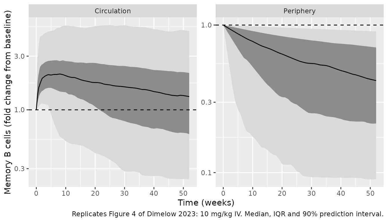
Dosing regimens (Figure 5a)
summ_circ <- sim |>
  group_by(treatment, time) |>
  summarise(p10 = quantile(fc, 0.1), med = median(fc), p90 = quantile(fc, 0.9),
            .groups = "drop")
ggplot(summ_circ, aes(time / 7)) +
  geom_line(aes(y = med), colour = "blue") +
  geom_line(aes(y = p10), colour = "red") +
  geom_line(aes(y = p90), colour = "red") +
  geom_hline(yintercept = 1, linetype = "dashed", colour = "blue") +
  scale_y_log10() +
  facet_wrap(~treatment) +
  labs(x = "Time (weeks)", y = "Memory B cells (fold change from baseline)",
       caption = "Replicates Figure 5a of Dimelow 2023: median and 10th / 90th percentiles of the individual predictions.")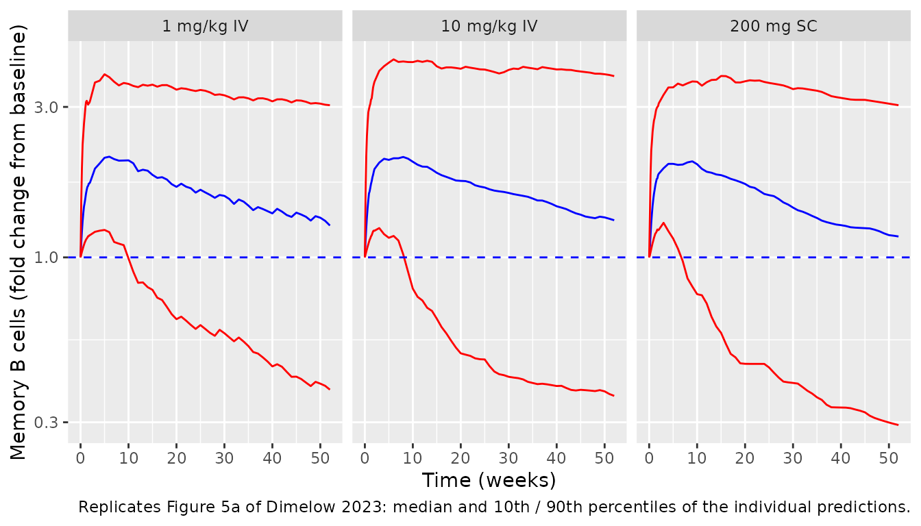
Comparison with the reported response
Reference values are from the Discussion (200 mg SC weekly: median fold-change 1.67 at week 1 and 2.21 at week 4) and, read off the figures by the maintainers, the 10 mg/kg IV medians of Figure 4.
pick <- function(trt, pan, day) {
  v <- summ$med[summ$treatment == trt & summ$panel == pan & summ$time == day]
  if (length(v) != 1L) stop("no unique row for ", trt, " / ", pan, " / day ", day)
  v
}
ref <- data.frame(
  quantity = c(
    "200 mg SC, circulating, week 1", "200 mg SC, circulating, week 4",
    "10 mg/kg IV, circulating, week 8", "10 mg/kg IV, circulating, week 52",
    "10 mg/kg IV, periphery, week 24", "10 mg/kg IV, periphery, week 52"
  ),
  source = c("Discussion", "Discussion", "Figure 4 (digitised)", "Figure 4 (digitised)",
             "Figure 4 (digitised)", "Figure 4 (digitised)"),
  # Figure 4 medians digitised on its log axes: circulation 2.27 (week 8) and
  # 1.27 (week 52); periphery 0.44 (week 24) and 0.31 (week 52).
  reported = c(1.67, 2.21, 2.27, 1.27, 0.44, 0.31),
  deviation = c(FALSE, FALSE, FALSE, FALSE, TRUE, TRUE),
  simulated = c(
    pick("200 mg SC", "Circulation", 7), pick("200 mg SC", "Circulation", 28),
    pick("10 mg/kg IV", "Circulation", 56), pick("10 mg/kg IV", "Circulation", 364),
    pick("10 mg/kg IV", "Periphery", 168), pick("10 mg/kg IV", "Periphery", 364)
  )
) |>
  mutate(pct_diff = round(100 * (simulated / reported - 1), 1),
         simulated = round(simulated, 2))
ref |>
  dplyr::rename("Median fold change" = quantity, Source = source,
                Reported = reported, Simulated = simulated, "% diff" = pct_diff,
                "Known deviation" = deviation) |>
knitr::kable()| Median fold change | Source | Reported | Known deviation | Simulated | % diff |
|---|---|---|---|---|---|
| 200 mg SC, circulating, week 1 | Discussion | 1.67 | FALSE | 1.59 | -4.8 |
| 200 mg SC, circulating, week 4 | Discussion | 2.21 | FALSE | 1.98 | -10.4 |
| 10 mg/kg IV, circulating, week 8 | Figure 4 (digitised) | 2.27 | FALSE | 2.08 | -8.3 |
| 10 mg/kg IV, circulating, week 52 | Figure 4 (digitised) | 1.27 | FALSE | 1.31 | 3.3 |
| 10 mg/kg IV, periphery, week 24 | Figure 4 (digitised) | 0.44 | TRUE | 0.59 | 34.0 |
| 10 mg/kg IV, periphery, week 52 | Figure 4 (digitised) | 0.31 | TRUE | 0.42 | 35.6 |
# Centre of the distribution only (no extremes). A mis-transcribed Emax, KM or
# ratio moves these medians by far more than 25%. The periphery rows are a
# known deviation (discussed below) and are reported but not gated.
stopifnot(all(abs(ref$pct_diff[!ref$deviation]) < 25))
The simulated circulating medians are within about 10% of the reported ones, mostly below them. The unobserved peripheral pool is depleted more slowly than in Figure 4: its median is about 35% above the figure at weeks 24 and 52. The typical-value subject is closer, with the peripheral pool at 0.52 at week 26 and 0.35 at week 52 for 10 mg/kg IV. The typical-value subject (median covariates, all etas zero) reaches a fold-change of about 2.5 at week 4, but the median across subjects is lower because of the large between-patient variability on KM (log-scale SD 1.16). Dimelow 2023 estimated a full correlation matrix for the four random effects (LKJ prior) but did not report it, so the etas here are independent. That is the most likely cause of the gap. It also means this model cannot reproduce Figure 5b, where patients with low baseline memory B cells have larger fold changes. With independent etas the fold change does not depend on MEMBL at all, so that dependence must come from a correlation between MEMBL and Emax and/or KM.
# Fold change vs baseline memory B cells (Figure 5b stratification): with
# independent etas the quartile medians are flat, unlike Figure 5b.
sim |>
  filter(treatment == "200 mg SC", time == 28) |>
  mutate(baseline_quartile = cut(rbase, c(0, 7, 15, 30, Inf),
                                 labels = c("<=7", "7-15", "15-30", ">30"))) |>
  group_by(baseline_quartile) |>
  summarise(n = n(), median_fc_week4 = round(median(fc), 2)) |>
knitr::kable()| baseline_quartile | n | median_fc_week4 |
|---|---|---|
| <=7 | 35 | 1.88 |
| 7-15 | 59 | 2.08 |
| 15-30 | 67 | 1.98 |
| >30 | 39 | 1.97 |
Assumptions and deviations
- Random-effect correlations not reported. Table 2 gives the log-scale SD of each random effect (posterior median), and the text says the correlation matrix had an LKJ(2) prior, but the posterior correlations are not published. The four etas are entered as independent with variance = SD^2. The consequences are discussed above. The circulating median fold change is up to about 10% low. The median peripheral pool is about 35% above Figure 4 and is excluded from the validation gate. The baseline dependence in Figure 5b is not reproduced.
- Posterior medians as point estimates. The packaged values are the Stan posterior medians of Table 2. Population predictions in the paper integrate over the posterior, so they are not exactly reproducible from point estimates.
-
PK typical values only. Following the paper, the PK
layer has no between-subject variability beyond body weight and BMI, and
all PK values are fixed. The SC V2 weight effect is printed as
(WT/67)in Table S1 and is entered with exponent 1. The source SC popPK paper (Struemper 2018, packaged asStruemper_2017_belimumab) fixed it at 0.8, and that model also has albumin and IgG effects on CL that Dimelow 2023 does not list. This model follows Table S1. Pediatric patients used the adult IV parameters, as in the paper. - Covariate distributions. The virtual cohort draws weight, BMI, BLyS and anti-dsDNA independently from log-normal distributions matched to Table S2 (pooled belimumab + placebo); correlations between covariates are ignored. The cohort is adult-only.
- Figure readings. The Figure 3b points and the Figure 4 medians in the comparison table were read off the published figures by the maintainers.
- Covariates screened but not retained. Body weight, BMI, age, baseline C3, C4 and SELENA-SLEDAI were screened against the week-8 simulated response (Table S3) and not retained for the memory B-cell parameters. Weight and BMI enter only through the PK.