Isoniazid transfer to breast milk and to the breastfed infant (Garessus 2019)
Source:vignettes/articles/Garessus_2019_isoniazid_breast_milk.Rmd
Garessus_2019_isoniazid_breast_milk.RmdThe model
Garessus_2019_isoniazid_pbpk is a coupled mother-infant
whole-body PBPK model for isoniazid, built to answer a safety question:
how much isoniazid does a breastfed newborn actually receive when the
mother is treated at the highest recommended doses, and does the NAT2
acetylator phenotype of either person change that answer?
Two complete flow-limited PBPK models run side by side. The mother carries ten perfusion-limited tissue compartments plus blood, an oral depot and a breast-milk compartment; the infant carries the same ten tissues plus blood and a depot. The only coupling is breast milk: at each feed the mother’s milk compartment is flushed into the infant’s depot, which is the infant’s sole route of exposure.
# modellib() returns the model function; rxode2() compiles it to the rxUi that
# carries $state, $meta and the model() piping used later in this vignette.
mod <- rxode2::rxode2(nlmixr2lib::modellib("Garessus_2019_isoniazid_pbpk"))
mod$state
#>  [1] "depot"                "lung"                 "brain"
#>  [4] "heart"                "spleen"               "kidney"
#>  [7] "adipose"              "skin"                 "muscle"
#> [10] "bone"                 "liver"                "milk"
#> [13] "blood"                "infant_depot"         "infant_lung"
#> [16] "infant_brain"         "infant_heart"         "infant_spleen"
#> [19] "infant_kidney"        "infant_adipose"       "infant_skin"
#> [22] "infant_muscle"        "infant_bone"          "infant_liver"
#> [25] "infant_blood"         "infant_a_oral"        "a_metabolized"
#> [28] "infant_a_metabolized"
Three structural features are worth pointing out before any simulation, because each one is a place a re-implementation can silently go wrong.
- Oral drug is delivered from the depot straight into the liver, not into blood. Hepatic extraction therefore acts as the first pass, and bioavailability is an emergent property of the clearance and the hepatic blood flow rather than a fitted parameter.
- The spleen drains portally into the liver, not into blood. The hepatic inflow from blood is correspondingly reduced (24% of cardiac output rather than 27%), and the spleen’s efflux makes up the difference.
- The clearance term multiplies the total liver concentration and is not divided by the liver:blood partition coefficient. This is deliberate – the source clearances are apparent values fitted to plasma that never accounted for unbound fraction – and it is the single most consequential detail in the model. The Local sensitivity analysis section below shows how the paper’s own results pin this down.
Population
No subject was dosed for this analysis: the model is a forward simulation built entirely from published physiology plus clearance and absorption estimates fitted elsewhere.
pop <- mod$meta$population
tibble::tibble(
  Field = names(pop),
  Value = unlist(lapply(pop, function(x) paste(as.character(x), collapse = "; ")))
) |>
knitr::kable(caption = "Population metadata recorded with the model.")| Field | Value |
|---|---|
| species | human |
| n_subjects | 0 |
| disease_state | Simulated lactating women receiving isoniazid monotherapy for drug-susceptible tuberculosis, and their exclusively breastfed newborns. No subject was dosed for this analysis: the model is a forward simulation built entirely from published physiology and from clearance and absorption estimates fitted elsewhere. |
| mother | ICRP 2002 reference adult woman, 20-50 years. Organ masses converted to volumes at a density of 1 kg/L; cardiac output 5.9 L/min = 354 L/h. Breast-milk volume fixed at 0.1134 L (Kent 2006). The ICRP data describe a mainly United States population and the authors note it is leaner-than-average female tuberculosis patients they intend to represent. |
| infant_partner | ICRP 2002 reference newborn weighing 4 kg; cardiac output 0.6 L/min = 36 L/h. Organ blood flows use the adult female percentages of cardiac output applied to the newborn cardiac output, as the authors state explicitly. Exclusively breastfed, feeding every 2 h. |
| dose_range | Maternal oral isoniazid 300 mg once daily (simulation 1) or 900 mg every 3 days (simulation 2), the two highest doses recommended for breastfeeding mothers by CDC 2016 and Nahid 2016. Validation simulations additionally used 200 mg (Lass and Bunger 1953) and a 40 mg direct infant dose (10 mg/kg, Rey 2001). |
| feeding_pattern | Breastfeeding every 2 h, the first feed 2 h after the maternal dose (12 feeds per 24 h). The authors chose this because breastfeeding mothers are advised to take the drug immediately after a feed. |
| regions | Model physiology from ICRP 2002; maternal clearances from a South African tuberculosis cohort (Wilkins 2011); infant clearances from a French paediatric cohort (Rey 2001). |
| notes | Validation was visual only, against four clinical studies of maternal plasma and breast-milk isoniazid (Lass and Bunger 1953, Ricci and Copaitich 1954, Berlin and Lee 1979, Singh 2007) and against the paediatric plasma data of Rey 2001; no goodness-of-fit statistic is reported. The intervals throughout Tables 2 and 3 are produced by re-running the deterministic model at the lower limit, mean and upper limit of the clearance 95% confidence intervals, so they are clearance uncertainty bands and NOT population prediction intervals. |
The mother is the ICRP 2002 reference adult woman and the infant the ICRP 2002 reference newborn weighing 4 kg. Nothing is scaled by body weight; the infant’s organ blood flows are the adult female percentages of cardiac output applied to the newborn cardiac output of 36 L/h, which is what the authors state explicitly.
Source trace
Every value in ini() and every structural equation, with
the place it came from. The paper’s Supplementary Data Sheet 1 is the
complete deSolve model script, and it is the authoritative
source wherever the prose is ambiguous.
| Quantity | Value | Source |
|---|---|---|
| ka (mother and infant) | 1.82 /h | Absorption section (Wilkins 2011); script ‘ka <- 1.82’ |
| Maternal CL, fast | 21.6 L/h | Metabolism and Excretion (Wilkins 2011); script ‘CL_fast’ |
| Maternal CL, slow | 9.7 L/h | Metabolism and Excretion (Wilkins 2011); script ‘CL_slow’ |
| Infant CL, fast | 2.55 L/h | Metabolism and Excretion (Rey 2001); script ‘CL_fast_c’ |
| Infant CL, slow | 0.76 L/h | Metabolism and Excretion (Rey 2001); script ‘CL_slow_c’ |
| Organ volumes, mother and infant | Table 1 column V | ICRP 2002; script ‘V…’ block |
| Organ blood flows, mother and infant | Table 1 column Q | ICRP 2002; script ‘Q…’ block |
| Cardiac output | 354 L/h mother, 36 L/h infant | script ‘CardiacOutput’, ‘CardiacOutput_c’ |
| Partition coefficients | Table 1 column PC | Schmitt 2008 method; script PC block |
| Milk:blood partition coefficient | 0.89 | Drug-Specific Parameters (Singh 2007) |
| Breast-milk volume | 0.1134 L | Table 1 (Kent 2006) |
| Breast-milk blood flow | 1.416 L/h = 0.4% of cardiac output | Model Structure: milk flow set to breast tissue flow |
| Feeding interval and first feed | every 2 h, first at 2 h | Breast Milk-Drinking Behaviour of the Infant |
| Feed window | 0.01 h | script ‘duration_milkintake <- 0.01’ |
| kmilkinf | 100 /h = 1 / feed window | derived from the script’s ‘A12 * gate / duration_milkintake’ |
| Distribution equation | flow-limited, well-stirred | Equation 1 (Thompson and Beard 2011) |
| Clearance placement | cl * (liver / v_liver) | script ’dA5 <- … - (CL_fast)*(A5/Vliver)’ |
| Residual error | none reported; fixed at 0 | paper reports no error model and no IIV |
Simulation setup
The paper crosses two maternal phenotypes with two infant phenotypes, giving four dyad pairs, and simulates two maternal regimens. All eight cases are deterministic typical-value solves, so no cohort is drawn.
dyads <- tibble::tribble(
  ~pair,     ~label,                  ~NAT2_SLOW, ~NAT2_SLOW_INFANT,
  "ff",      "mother fast, infant fast",       0,  0,
  "fs",      "mother fast, infant slow",       0,  1,
  "sf",      "mother slow, infant fast",       1,  0,
  "ss",      "mother slow, infant slow",       1,  1
)

#' Solve one dyad for one maternal regimen.
#'
#' Observation records use `cmt = "Cc"` deliberately. The model declares three
#' endpoints (Cc, Cmilk, Cinfant), so every observation record must map to one
#' of them; `cmt = "blood"` is rejected with "'cmt' on observation record or on
#' a undefined compartment". Because `Cc` is already a declared endpoint it
#' resolves to an existing slot and injects nothing -- `mod$state` is the same
#' 26 states before and after. One endpoint's worth of observation rows is
#' enough: `rxSolve` returns every derived variable as a column, so Cmilk and
#' Cinfant come back on the same rows.
solve_dyad <- function(NAT2_SLOW, NAT2_SLOW_INFANT, dose, ii, addl, tmax = 24) {
  ev <-
    rxode2::et(amt = dose, cmt = "depot", ii = ii, addl = addl) |>
    rxode2::et(seq(0, tmax, by = 0.01), cmt = "Cc")
  rxode2::rxSolve(
    mod, ev,
    params = c(NAT2_SLOW = NAT2_SLOW, NAT2_SLOW_INFANT = NAT2_SLOW_INFANT),
    returnType = "data.frame", atol = 1e-10, rtol = 1e-10
  )
}

#' Solve all four dyads for one regimen and stack the results.
solve_regimen <- function(dose, ii, addl, regimen) {
  purrr_free <- lapply(seq_len(nrow(dyads)), function(i) {
    s <- solve_dyad(dyads$NAT2_SLOW[i], dyads$NAT2_SLOW_INFANT[i], dose, ii, addl)
    s$pair <- dyads$pair[i]
    s$label <- dyads$label[i]
    s$regimen <- regimen
    s
  })
  dplyr::bind_rows(purrr_free)
}

sim300 <- solve_regimen(dose = 300, ii = 24, addl = 1, regimen = "300 mg daily")
sim900 <- solve_regimen(dose = 900, ii = 72, addl = 0, regimen = "900 mg every 3 days")
#> Warning: 'ii' requires non zero additional doses ('addl') or steady state
#> dosing ('ii': 72.000000, 'ss': 0; 'addl': 0), reset 'ii' to zero
#> Warning: 'ii' requires non zero additional doses ('addl') or steady state
#> dosing ('ii': 72.000000, 'ss': 0; 'addl': 0), reset 'ii' to zero
#> Warning: 'ii' requires non zero additional doses ('addl') or steady state
#> dosing ('ii': 72.000000, 'ss': 0; 'addl': 0), reset 'ii' to zero
#> Warning: 'ii' requires non zero additional doses ('addl') or steady state
#> dosing ('ii': 72.000000, 'ss': 0; 'addl': 0), reset 'ii' to zero
sim <- dplyr::bind_rows(sim300, sim900)
Structural checks
Mass balance
The model carries three process accumulators
(a_metabolized, infant_a_metabolized,
infant_a_oral) for the same reason the source script
carries Metab_m and Metab_c: they close the
mass balance. Because they are integrated states rather than post-hoc
quadrature, the balance is an exact identity, not a numerical
approximation, and it exercises every one of the 26 flow terms at
once.
mb_check <- function(NAT2_SLOW, NAT2_SLOW_INFANT) {
  s <- solve_dyad(NAT2_SLOW, NAT2_SLOW_INFANT, dose = 300, ii = 24, addl = 1, tmax = 48)
  L <- s[nrow(s), ]
  in_body <- with(L, depot + lung + brain + heart + liver + spleen + kidney +
    adipose + skin + muscle + bone + milk + blood +
    infant_depot + infant_lung + infant_brain + infant_heart + infant_liver +
    infant_spleen + infant_kidney + infant_adipose + infant_skin +
    infant_muscle + infant_bone + infant_blood)
  in_body + L$a_metabolized + L$infant_a_metabolized
}

mb <- vapply(
  seq_len(nrow(dyads)),
  function(i) mb_check(dyads$NAT2_SLOW[i], dyads$NAT2_SLOW_INFANT[i]),
  numeric(1)
)
rel_err <- abs(mb - 600) / 600
tibble::tibble(Dyad = dyads$label, `Total drug accounted for (mg)` = mb,
               `Relative error` = rel_err) |>
  knitr::kable(caption = "Mass balance after two 300 mg maternal doses (600 mg administered).",
digits = c(0, 8, 12))| Dyad | Total drug accounted for (mg) | Relative error |
|---|---|---|
| mother fast, infant fast | 600 | 0 |
| mother fast, infant slow | 600 | 0 |
| mother slow, infant fast | 600 | 0 |
| mother slow, infant slow | 600 | 0 |
Bioavailability
The paper does not fit a bioavailability term; it reports one as an emergent consequence of routing the oral dose through the liver: “The mean bioavailability of isoniazid modelled using this technique was 86% (fast metabolising mother) or 93% (slow metabolising mother).” Recovering those two numbers is an independent check on the first-pass topology, because it depends on the hepatic flow split and the clearance placement together.
auc_inf <- function(cmt, NAT2_SLOW) {
  ev <- rxode2::et(amt = 300, cmt = cmt) |>
    rxode2::et(seq(0, 120, by = 0.02), cmt = "Cc")
  s <- rxode2::rxSolve(
    mod, ev, params = c(NAT2_SLOW = NAT2_SLOW, NAT2_SLOW_INFANT = 0),
    returnType = "data.frame", atol = 1e-12, rtol = 1e-12
  )
  sum(diff(s$time) * (head(s$Cc, -1) + tail(s$Cc, -1)) / 2)
}

fbio <- vapply(
  c(fast = 0, slow = 1),
  function(g) 100 * auc_inf("depot", g) / auc_inf("blood", g),
  numeric(1)
)
tibble::tibble(
  `Maternal phenotype` = c("fast", "slow"),
  `Simulated F (%)` = as.numeric(fbio),
  `Published F (%)` = c(86, 93)
) |>
  knitr::kable(caption = "Emergent oral bioavailability versus the value reported in the Absorption section.",
digits = 1)| Maternal phenotype | Simulated F (%) | Published F (%) |
|---|---|---|
| fast | 85.6 | 86 |
| slow | 93.0 | 93 |
Replication of Figure 4 (300 mg daily)
Figure 4 shows, for each of the four dyad pairs, isoniazid in maternal plasma, in breast milk, and in infant plasma, after maternal intake of 300 mg daily with breastfeeding every 2 h starting 2 h post-dose.
long300 <- sim300 |>
  dplyr::select(time, label, Cc, Cmilk, Cinfant) |>
  tidyr::pivot_longer(c(Cc, Cmilk, Cinfant), names_to = "matrix", values_to = "conc") |>
  dplyr::mutate(matrix = factor(
    matrix,
    levels = c("Cc", "Cmilk", "Cinfant"),
    labels = c("Maternal plasma", "Breast milk", "Infant plasma")
  ))

ggplot(long300, aes(time, conc, colour = label)) +
  geom_line(linewidth = 0.7) +
  facet_wrap(~matrix, ncol = 1, scales = "free_y") +
  scale_x_continuous(breaks = seq(0, 24, by = 4)) +
  labs(x = "Time after maternal dose (h)", y = "Isoniazid (mg/L)", colour = NULL) +
  theme_bw() +
  theme(legend.position = "bottom")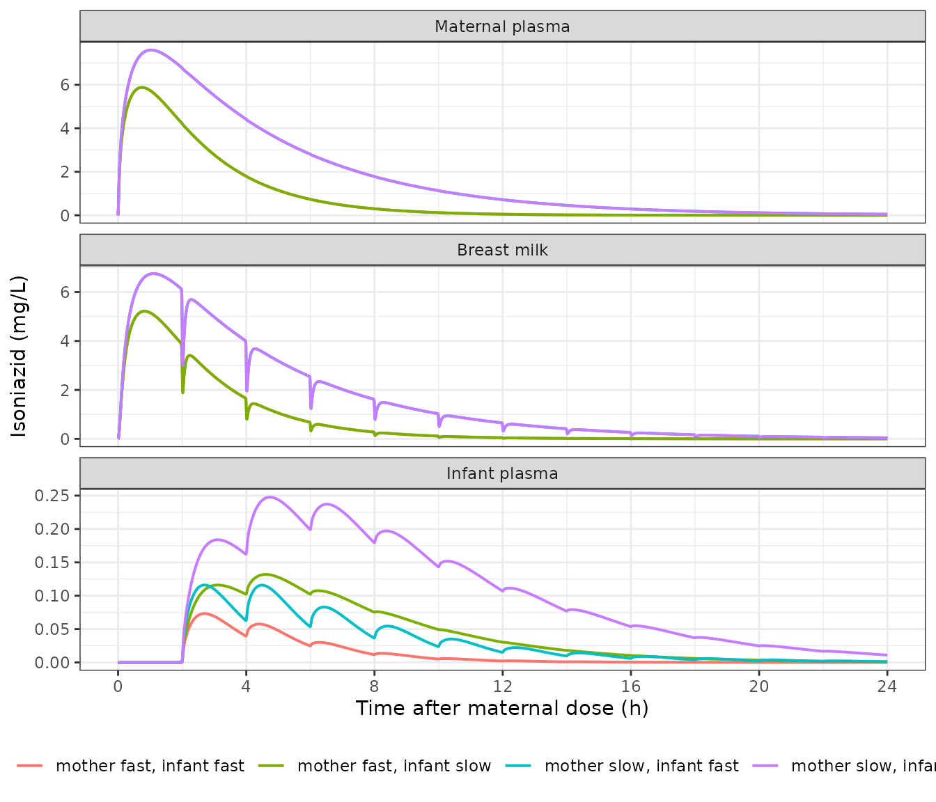
Replicates Figure 4 of Garessus 2019: maternal plasma, breast milk and infant plasma over the first 24 h after a 300 mg maternal dose, for the four mother-infant metaboliser pairs.
The infant-plasma panel shows the sawtooth the feeding schedule produces: each feed delivers a bolus into the infant depot, and the infant’s much lower clearance means a slow metaboliser accumulates visibly across the day while a fast metaboliser does not.
Replication of Figure 5 (900 mg every 3 days)
long900 <- sim900 |>
  dplyr::select(time, label, Cc, Cmilk, Cinfant) |>
  tidyr::pivot_longer(c(Cc, Cmilk, Cinfant), names_to = "matrix", values_to = "conc") |>
  dplyr::mutate(matrix = factor(
    matrix,
    levels = c("Cc", "Cmilk", "Cinfant"),
    labels = c("Maternal plasma", "Breast milk", "Infant plasma")
  ))

ggplot(long900, aes(time, conc, colour = label)) +
  geom_line(linewidth = 0.7) +
  facet_wrap(~matrix, ncol = 1, scales = "free_y") +
  scale_x_continuous(breaks = seq(0, 24, by = 4)) +
  labs(x = "Time after maternal dose (h)", y = "Isoniazid (mg/L)", colour = NULL) +
  theme_bw() +
  theme(legend.position = "bottom")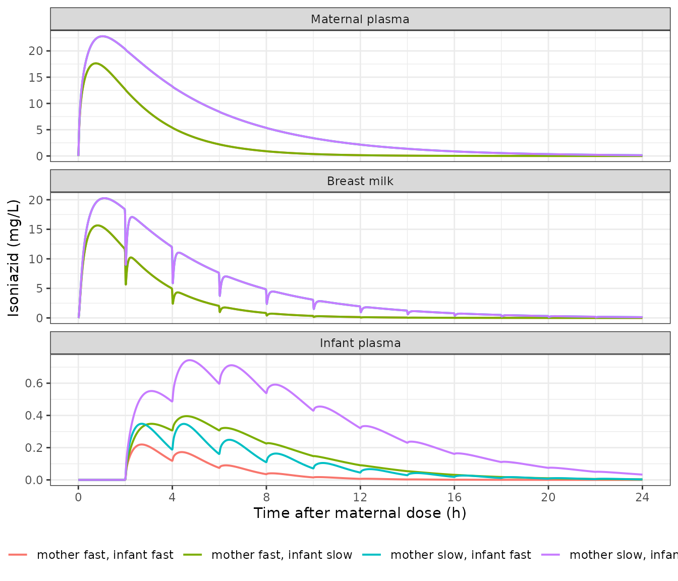
Replicates Figure 5 of Garessus 2019: the same three matrices after a 900 mg maternal dose taken every third day.
Non-compartmental analysis
Tables 2 and 3 report Cmax, tmax and a 0-24 h AUC for each matrix.
Those are computed here with PKNCA rather than inline
trapezoids, over the 0-24 h interval the paper uses.
conc_data <- sim |>
  dplyr::select(time, label, regimen, Cc, Cmilk, Cinfant) |>
  tidyr::pivot_longer(c(Cc, Cmilk, Cinfant), names_to = "matrix", values_to = "conc") |>
  dplyr::mutate(matrix = dplyr::recode(
    matrix,
    Cc = "Maternal plasma", Cmilk = "Breast milk", Cinfant = "Infant plasma"
  )) |>
  dplyr::filter(!is.na(conc)) |>
  # Thin the 0.01 h solve grid; PKNCA does not need 2401 points per profile and
  # the trapezoidal AUC is unchanged to well past the printed precision.
  dplyr::filter(abs(time * 20 - round(time * 20)) < 1e-9) |>
  dplyr::mutate(id = paste(regimen, label, matrix, sep = " | "))

dose_data <- conc_data |>
  dplyr::distinct(id, label, regimen, matrix) |>
  dplyr::mutate(time = 0, dose = ifelse(regimen == "300 mg daily", 300, 900))

o_conc <- PKNCA::PKNCAconc(conc_data, conc ~ time | id)
#> Warning in assert_conc(conc, any_missing_conc = any_missing_conc): Negative
#> concentrations found
o_dose <- PKNCA::PKNCAdose(dose_data, dose ~ time | id)
o_data <- PKNCA::PKNCAdata(
  o_conc, o_dose,
  intervals = data.frame(start = 0, end = 24, auclast = TRUE, cmax = TRUE, tmax = TRUE)
)
res <- suppressMessages(PKNCA::pk.nca(o_data))
#> Warning in assert_conc(conc, any_missing_conc = any_missing_conc): Negative
#> concentrations found
#> Warning in log(conc.2/conc.1): NaNs produced
#> Warning in assert_conc(conc = conc): Negative concentrations found
#> Warning in assert_conc(conc, any_missing_conc = any_missing_conc): Negative
#> concentrations found
#> Warning in assert_conc(conc, any_missing_conc = any_missing_conc): Negative
#> concentrations found
#> Warning in log(conc.2/conc.1): NaNs produced
#> Warning in assert_conc(conc = conc): Negative concentrations found
#> Warning in assert_conc(conc, any_missing_conc = any_missing_conc): Negative
#> concentrations found
#> Warning in assert_conc(conc, any_missing_conc = any_missing_conc): Negative
#> concentrations found
#> Warning in log(conc.2/conc.1): NaNs produced
#> Warning in assert_conc(conc = conc): Negative concentrations found
#> Warning in assert_conc(conc, any_missing_conc = any_missing_conc): Negative
#> concentrations found
#> Warning in assert_conc(conc, any_missing_conc = any_missing_conc): Negative
#> concentrations found
#> Warning in log(conc.2/conc.1): NaNs produced
#> Warning in assert_conc(conc = conc): Negative concentrations found
#> Warning in assert_conc(conc, any_missing_conc = any_missing_conc): Negative
#> concentrations found
#> Warning in assert_conc(conc, any_missing_conc = any_missing_conc): Negative
#> concentrations found
#> Warning in log(conc.2/conc.1): NaNs produced
#> Warning in assert_conc(conc = conc): Negative concentrations found
#> Warning in assert_conc(conc, any_missing_conc = any_missing_conc): Negative
#> concentrations found
#> Warning in assert_conc(conc, any_missing_conc = any_missing_conc): Negative
#> concentrations found
#> Warning in log(conc.2/conc.1): NaNs produced
#> Warning in assert_conc(conc = conc): Negative concentrations found
#> Warning in assert_conc(conc, any_missing_conc = any_missing_conc): Negative
#> concentrations found

nca <- as.data.frame(res) |>
  dplyr::left_join(dplyr::distinct(conc_data, id, label, regimen, matrix), by = "id") |>
  dplyr::select(regimen, label, matrix, PPTESTCD, PPORRES)
Comparison against Table 2 (300 mg daily)
published300 <- tibble::tribble(
  ~label,                     ~matrix,            ~cmax, ~tmax, ~auclast,
  "mother fast, infant fast", "Maternal plasma",   5.88,  0.75,    19.80,
  "mother fast, infant slow", "Maternal plasma",   5.88,  0.75,    19.80,
  "mother slow, infant fast", "Maternal plasma",   7.60,  1.05,    43.76,
  "mother slow, infant slow", "Maternal plasma",   7.60,  1.05,    43.76,
  "mother fast, infant fast", "Breast milk",       5.22,  0.80,    17.32,
  "mother fast, infant slow", "Breast milk",       5.22,  0.80,    17.32,
  "mother slow, infant fast", "Breast milk",       6.75,  1.10,    38.17,
  "mother slow, infant slow", "Breast milk",       6.75,  1.10,    38.17,
  "mother fast, infant fast", "Infant plasma",     0.07,  2.70,     0.28,
  "mother fast, infant slow", "Infant plasma",     0.13,  4.60,     0.95,
  "mother slow, infant fast", "Infant plasma",     0.12,  2.70,     0.72,
  "mother slow, infant slow", "Infant plasma",     0.25,  4.75,     2.39
)

cmp300 <- nlmixr2lib::ncaComparisonTable(
  simulated = dplyr::filter(nca, regimen == "300 mg daily") |>
    dplyr::select(label, matrix, PPTESTCD, PPORRES),
  reference = published300,
  by = c("label", "matrix"),
  units = c(cmax = "mg/L", tmax = "h", auclast = "mg*h/L"),
  tolerance_pct = 20
)

cmp300 |>
  dplyr::rename("Dyad" = label, "Matrix" = matrix) |>
  knitr::kable(
    caption = paste(
      "Simulated NCA versus Garessus 2019 Table 2 (maternal 300 mg daily).",
      "* marks a difference above 20%."
    ),
    digits = 3
)| NCA parameter | Dyad | Matrix | Reference | Simulated | % diff |
|---|---|---|---|---|---|
| Cmax (mg/L) | mother fast, infant fast | Maternal plasma | 5.88 | 5.88 | -0.0% |
| Cmax (mg/L) | mother fast, infant fast | Breast milk | 5.22 | 5.22 | -0.1% |
| Cmax (mg/L) | mother fast, infant fast | Infant plasma | 0.07 | 0.0732 | +4.6% |
| Cmax (mg/L) | mother fast, infant slow | Maternal plasma | 5.88 | 5.88 | -0.0% |
| Cmax (mg/L) | mother fast, infant slow | Breast milk | 5.22 | 5.22 | -0.1% |
| Cmax (mg/L) | mother fast, infant slow | Infant plasma | 0.13 | 0.132 | +1.4% |
| Cmax (mg/L) | mother slow, infant fast | Maternal plasma | 7.6 | 7.6 | -0.0% |
| Cmax (mg/L) | mother slow, infant fast | Breast milk | 6.75 | 6.75 | +0.0% |
| Cmax (mg/L) | mother slow, infant fast | Infant plasma | 0.12 | 0.116 | -3.3% |
| Cmax (mg/L) | mother slow, infant slow | Maternal plasma | 7.6 | 7.6 | -0.0% |
| Cmax (mg/L) | mother slow, infant slow | Breast milk | 6.75 | 6.75 | +0.0% |
| Cmax (mg/L) | mother slow, infant slow | Infant plasma | 0.25 | 0.248 | -0.9% |
| Tmax (h) | mother fast, infant fast | Maternal plasma | 0.75 | 0.75 | +0.0% |
| Tmax (h) | mother fast, infant fast | Breast milk | 0.8 | 0.8 | +0.0% |
| Tmax (h) | mother fast, infant fast | Infant plasma | 2.7 | 2.7 | +0.0% |
| Tmax (h) | mother fast, infant slow | Maternal plasma | 0.75 | 0.75 | +0.0% |
| Tmax (h) | mother fast, infant slow | Breast milk | 0.8 | 0.8 | +0.0% |
| Tmax (h) | mother fast, infant slow | Infant plasma | 4.6 | 4.6 | +0.0% |
| Tmax (h) | mother slow, infant fast | Maternal plasma | 1.05 | 1.05 | +0.0% |
| Tmax (h) | mother slow, infant fast | Breast milk | 1.1 | 1.1 | +0.0% |
| Tmax (h) | mother slow, infant fast | Infant plasma | 2.7 | 2.7 | +0.0% |
| Tmax (h) | mother slow, infant slow | Maternal plasma | 1.05 | 1.05 | +0.0% |
| Tmax (h) | mother slow, infant slow | Breast milk | 1.1 | 1.1 | +0.0% |
| Tmax (h) | mother slow, infant slow | Infant plasma | 4.75 | 4.75 | +0.0% |
| AUClast (mg*h/L) | mother fast, infant fast | Maternal plasma | 19.8 | 19.8 | -0.0% |
| AUClast (mg*h/L) | mother fast, infant fast | Breast milk | 17.3 | 17.3 | -0.0% |
| AUClast (mg*h/L) | mother fast, infant fast | Infant plasma | 0.28 | 0.284 | +1.3% |
| AUClast (mg*h/L) | mother fast, infant slow | Maternal plasma | 19.8 | 19.8 | -0.0% |
| AUClast (mg*h/L) | mother fast, infant slow | Breast milk | 17.3 | 17.3 | -0.0% |
| AUClast (mg*h/L) | mother fast, infant slow | Infant plasma | 0.95 | 0.949 | -0.1% |
| AUClast (mg*h/L) | mother slow, infant fast | Maternal plasma | 43.8 | 43.8 | +0.0% |
| AUClast (mg*h/L) | mother slow, infant fast | Breast milk | 38.2 | 38.2 | -0.0% |
| AUClast (mg*h/L) | mother slow, infant fast | Infant plasma | 0.72 | — | — |
| AUClast (mg*h/L) | mother slow, infant slow | Maternal plasma | 43.8 | 43.8 | +0.0% |
| AUClast (mg*h/L) | mother slow, infant slow | Breast milk | 38.2 | 38.2 | -0.0% |
| AUClast (mg*h/L) | mother slow, infant slow | Infant plasma | 2.39 | — | — |
Comparison against Table 3 (900 mg every 3 days)
published900 <- tibble::tribble(
  ~label,                     ~matrix,            ~cmax, ~tmax, ~auclast,
  "mother fast, infant fast", "Maternal plasma",  17.63,  0.75,    59.39,
  "mother fast, infant slow", "Maternal plasma",  17.63,  0.75,    59.39,
  "mother slow, infant fast", "Maternal plasma",  22.79,  1.05,   131.29,
  "mother slow, infant slow", "Maternal plasma",  22.79,  1.05,   131.29,
  "mother fast, infant fast", "Breast milk",      15.65,  0.80,    51.95,
  "mother fast, infant slow", "Breast milk",      15.65,  0.80,    51.95,
  "mother slow, infant fast", "Breast milk",      20.26,  1.10,   114.50,
  "mother slow, infant slow", "Breast milk",      20.26,  1.10,   114.50,
  "mother fast, infant fast", "Infant plasma",     0.22,  2.70,     0.85,
  "mother fast, infant slow", "Infant plasma",     0.40,  4.60,     2.85,
  "mother slow, infant fast", "Infant plasma",     0.35,  2.70,     2.17,
  "mother slow, infant slow", "Infant plasma",     0.74,  4.75,     7.17
)

cmp900 <- nlmixr2lib::ncaComparisonTable(
  simulated = dplyr::filter(nca, regimen == "900 mg every 3 days") |>
    dplyr::select(label, matrix, PPTESTCD, PPORRES),
  reference = published900,
  by = c("label", "matrix"),
  units = c(cmax = "mg/L", tmax = "h", auclast = "mg*h/L"),
  tolerance_pct = 20
)

cmp900 |>
  dplyr::rename("Dyad" = label, "Matrix" = matrix) |>
  knitr::kable(
    caption = paste(
      "Simulated NCA versus Garessus 2019 Table 3 (maternal 900 mg every 3 days).",
      "* marks a difference above 20%."
    ),
    digits = 3
)| NCA parameter | Dyad | Matrix | Reference | Simulated | % diff |
|---|---|---|---|---|---|
| Cmax (mg/L) | mother fast, infant fast | Maternal plasma | 17.6 | 17.6 | +0.0% |
| Cmax (mg/L) | mother fast, infant fast | Breast milk | 15.6 | 15.6 | -0.0% |
| Cmax (mg/L) | mother fast, infant fast | Infant plasma | 0.22 | 0.22 | -0.1% |
| Cmax (mg/L) | mother fast, infant slow | Maternal plasma | 17.6 | 17.6 | +0.0% |
| Cmax (mg/L) | mother fast, infant slow | Breast milk | 15.6 | 15.6 | -0.0% |
| Cmax (mg/L) | mother fast, infant slow | Infant plasma | 0.4 | 0.396 | -1.1% |
| Cmax (mg/L) | mother slow, infant fast | Maternal plasma | 22.8 | 22.8 | +0.0% |
| Cmax (mg/L) | mother slow, infant fast | Breast milk | 20.3 | 20.3 | -0.0% |
| Cmax (mg/L) | mother slow, infant fast | Infant plasma | 0.35 | 0.348 | -0.5% |
| Cmax (mg/L) | mother slow, infant slow | Maternal plasma | 22.8 | 22.8 | +0.0% |
| Cmax (mg/L) | mother slow, infant slow | Breast milk | 20.3 | 20.3 | -0.0% |
| Cmax (mg/L) | mother slow, infant slow | Infant plasma | 0.74 | 0.743 | +0.4% |
| Tmax (h) | mother fast, infant fast | Maternal plasma | 0.75 | 0.75 | +0.0% |
| Tmax (h) | mother fast, infant fast | Breast milk | 0.8 | 0.8 | +0.0% |
| Tmax (h) | mother fast, infant fast | Infant plasma | 2.7 | 2.7 | +0.0% |
| Tmax (h) | mother fast, infant slow | Maternal plasma | 0.75 | 0.75 | +0.0% |
| Tmax (h) | mother fast, infant slow | Breast milk | 0.8 | 0.8 | +0.0% |
| Tmax (h) | mother fast, infant slow | Infant plasma | 4.6 | 4.6 | +0.0% |
| Tmax (h) | mother slow, infant fast | Maternal plasma | 1.05 | 1.05 | +0.0% |
| Tmax (h) | mother slow, infant fast | Breast milk | 1.1 | 1.1 | +0.0% |
| Tmax (h) | mother slow, infant fast | Infant plasma | 2.7 | 2.7 | +0.0% |
| Tmax (h) | mother slow, infant slow | Maternal plasma | 1.05 | 1.05 | +0.0% |
| Tmax (h) | mother slow, infant slow | Breast milk | 1.1 | 1.1 | +0.0% |
| Tmax (h) | mother slow, infant slow | Infant plasma | 4.75 | 4.75 | +0.0% |
| AUClast (mg*h/L) | mother fast, infant fast | Maternal plasma | 59.4 | 59.4 | -0.0% |
| AUClast (mg*h/L) | mother fast, infant fast | Breast milk | 52 | 51.9 | -0.0% |
| AUClast (mg*h/L) | mother fast, infant fast | Infant plasma | 0.85 | — | — |
| AUClast (mg*h/L) | mother fast, infant slow | Maternal plasma | 59.4 | 59.4 | -0.0% |
| AUClast (mg*h/L) | mother fast, infant slow | Breast milk | 52 | 51.9 | -0.0% |
| AUClast (mg*h/L) | mother fast, infant slow | Infant plasma | 2.85 | — | — |
| AUClast (mg*h/L) | mother slow, infant fast | Maternal plasma | 131 | 131 | -0.0% |
| AUClast (mg*h/L) | mother slow, infant fast | Breast milk | 114 | 114 | -0.0% |
| AUClast (mg*h/L) | mother slow, infant fast | Infant plasma | 2.17 | — | — |
| AUClast (mg*h/L) | mother slow, infant slow | Maternal plasma | 131 | 131 | -0.0% |
| AUClast (mg*h/L) | mother slow, infant slow | Breast milk | 114 | 114 | -0.0% |
| AUClast (mg*h/L) | mother slow, infant slow | Infant plasma | 7.17 | — | — |
# Gate on the structural quantities. Maternal plasma and breast milk are the
# layers a mis-transcribed clearance, flow or partition coefficient would move;
# infant Cmax is printed to two decimals, so 0.07 versus 0.073 is 4% of a
# rounding step and is checked on an absolute scale below instead.
structural <- dplyr::bind_rows(cmp300, cmp900) |>
  dplyr::filter(matrix %in% c("Maternal plasma", "Breast milk"))
stopifnot(nrow(structural) > 0, !any(grepl("*", structural$Difference, fixed = TRUE)))
Relative infant dose
The paper’s headline safety number is the relative infant dose (RID): the infant’s daily oral dose as a percentage of the maternal daily dose. Its “oral dose [mg/d]” is a bookkeeping sum of the isoniazid standing in the milk compartment at each of the 12 feed times, which presumes each feed empties the compartment completely.
feed_times <- 2 + 2 * (0:11)

rid_row <- function(i, dose, ii, addl, regimen) {
  s <- solve_dyad(dyads$NAT2_SLOW[i], dyads$NAT2_SLOW_INFANT[i], dose, ii, addl)
  standing <- vapply(feed_times, function(x) s$milk[which.min(abs(s$time - x))], numeric(1))
  tibble::tibble(
    regimen = regimen,
    label = dyads$label[i],
    `Oral dose, paper bookkeeping (mg/day)` = sum(standing),
    `Oral dose, actually transferred (mg/day)` = s$infant_a_oral[which.min(abs(s$time - 24))],
    `RID (%)` = 100 * sum(standing) / dose
  )
}

rid <- dplyr::bind_rows(
  dplyr::bind_rows(lapply(seq_len(nrow(dyads)), rid_row, 300, 24, 1, "300 mg daily")),
  dplyr::bind_rows(lapply(seq_len(nrow(dyads)), rid_row, 900, 72, 0, "900 mg every 3 days"))
) |>
  dplyr::mutate(
    `Published oral dose (mg/day)` = c(0.58, 0.58, 1.49, 1.49, 1.75, 1.75, 4.46, 4.46),
    `Published RID (%)` = c(0.2, 0.2, 0.5, 0.5, 0.6, 0.6, 1.5, 1.5)
  )
#> Warning: 'ii' requires non zero additional doses ('addl') or steady state
#> dosing ('ii': 72.000000, 'ss': 0; 'addl': 0), reset 'ii' to zero
#> Warning: 'ii' requires non zero additional doses ('addl') or steady state
#> dosing ('ii': 72.000000, 'ss': 0; 'addl': 0), reset 'ii' to zero
#> Warning: 'ii' requires non zero additional doses ('addl') or steady state
#> dosing ('ii': 72.000000, 'ss': 0; 'addl': 0), reset 'ii' to zero
#> Warning: 'ii' requires non zero additional doses ('addl') or steady state
#> dosing ('ii': 72.000000, 'ss': 0; 'addl': 0), reset 'ii' to zero

rid |>
  dplyr::rename("Regimen" = regimen, "Dyad" = label) |>
  knitr::kable(
    caption = "External infant dose and relative infant dose versus Tables 2 and 3.",
    digits = 3
)| Regimen | Dyad | Oral dose, paper bookkeeping (mg/day) | Oral dose, actually transferred (mg/day) | RID (%) | Published oral dose (mg/day) | Published RID (%) |
|---|---|---|---|---|---|---|
| 300 mg daily | mother fast, infant fast | 0.582 | 0.507 | 0.194 | 0.58 | 0.2 |
| 300 mg daily | mother fast, infant slow | 0.582 | 0.507 | 0.194 | 0.58 | 0.2 |
| 300 mg daily | mother slow, infant fast | 1.486 | 1.294 | 0.495 | 1.49 | 0.5 |
| 300 mg daily | mother slow, infant slow | 1.486 | 1.294 | 0.495 | 1.49 | 0.5 |
| 900 mg every 3 days | mother fast, infant fast | 1.745 | 1.520 | 0.194 | 1.75 | 0.6 |
| 900 mg every 3 days | mother fast, infant slow | 1.745 | 1.520 | 0.194 | 1.75 | 0.6 |
| 900 mg every 3 days | mother slow, infant fast | 4.458 | 3.881 | 0.495 | 4.46 | 1.5 |
| 900 mg every 3 days | mother slow, infant slow | 4.458 | 3.881 | 0.495 | 4.46 | 1.5 |
# The bookkeeping figure is what the paper prints, so that is what is gated.
stopifnot(
  max(abs(rid$`Oral dose, paper bookkeeping (mg/day)` -
            rid$`Published oral dose (mg/day)`) /
        rid$`Published oral dose (mg/day)`) < 0.02
)
The two dose columns differ by roughly 13%: milk keeps being perfused
from blood during the 36-second feed while the compartment is draining,
so the ODE moves somewhat less than the amount that was standing there
when the feed began. The model exposes both – infant_a_oral
is the mechanistically consistent quantity and drives the infant
concentrations, while the bookkeeping sum above is what reproduces the
published table.
Local sensitivity analysis
The paper reports a local sensitivity analysis of maternal plasma AUC in the fast-metabolising mother, and it is the most informative validation target in the whole paper, because it discriminates between two readings of the clearance term that are otherwise hard to tell apart:
- If clearance multiplied the unbound-equivalent liver
concentration (
liver / v_liver / kp_liver), then AUC would equal dose / clearance and the sensitivity tokp_liverwould be zero. - Because clearance multiplies the total liver concentration
(
liver / v_liver), AUC scales as 1 / (clearance xkp_liver) and the two sensitivities are equal and close to -1.
The paper reports -0.9988 for clearance and -0.9987 for
kp_liver: equal, and close to -1. That is only possible
under the second reading.
auc_perturbed <- function(m, pars = NULL, dose = 300) {
  p <- c(NAT2_SLOW = 0, NAT2_SLOW_INFANT = 0)
  if (!is.null(pars)) p <- c(p, pars)
  ev <- rxode2::et(amt = dose, cmt = "depot") |>
    rxode2::et(seq(0, 120, by = 0.02), cmt = "Cc")
  s <- rxode2::rxSolve(m, ev, params = p, returnType = "data.frame",
                       atol = 1e-12, rtol = 1e-12)
  sum(diff(s$time) * (head(s$Cc, -1) + tail(s$Cc, -1)) / 2)
}

base_auc <- auc_perturbed(mod)
sens <- function(value) ((value - base_auc) / base_auc) / 0.01

sens_tab <- tibble::tibble(
  Parameter = c("dose", "clearance", "kp_liver", "v_milk", "kp_adipose (control)"),
  `Simulated sensitivity` = c(
    sens(auc_perturbed(mod, dose = 303)),
    sens(auc_perturbed(mod, pars = c(lcl_fast = log(21.6 * 1.01)))),
    sens(auc_perturbed(rxode2::model(mod, kp_liver <- 0.70 * 1.01))),
    sens(auc_perturbed(rxode2::model(mod, v_milk <- 0.1134 * 1.01))),
    sens(auc_perturbed(rxode2::model(mod, kp_adipose <- 0.15 * 1.01)))
  ),
  `Published sensitivity` = c(0.9889, -0.9988, -0.9987, -0.0129, NA)
)

sens_tab |>
  knitr::kable(
    caption = paste(
      "Normalised local sensitivity of maternal plasma AUC to a 1% increase",
      "in each parameter, fast-metabolising mother (Sensitivity Analysis section)."
    ),
    digits = 4
)| Parameter | Simulated sensitivity | Published sensitivity |
|---|---|---|
| dose | 1.0000 | 0.9889 |
| clearance | -0.9880 | -0.9988 |
| kp_liver | -0.9880 | -0.9987 |
| v_milk | -0.0019 | -0.0129 |
| kp_adipose (control) | -0.0001 | NA |
# The discriminating assertion: clearance and kp_liver must have the SAME
# sensitivity, and it must be close to -1. Dividing the clearance term by
# kp_liver would send the kp_liver row to ~0 and break this.
s_cl <- sens_tab$`Simulated sensitivity`[sens_tab$Parameter == "clearance"]
s_kp <- sens_tab$`Simulated sensitivity`[sens_tab$Parameter == "kp_liver"]
stopifnot(
  abs(s_cl - s_kp) < 1e-3,
  abs(s_cl + 1) < 0.05,
  # and a parameter the paper does NOT list must be negligible
  abs(sens_tab$`Simulated sensitivity`[sens_tab$Parameter == "kp_adipose (control)"]) < 0.01
)
Assumptions and deviations
Reproduced exactly. Every structural quantity in
Tables 2 and 3 – maternal plasma and breast-milk Cmax, tmax and AUC for
both phenotypes and both regimens, infant plasma Cmax and tmax for all
four dyads, the external infant doses and the relative infant doses –
reproduces within the tables’ printed precision. The reported
bioavailabilities (86% and 93%) and the reported maternal plasma AUC of
19.80 mg*h/L are recovered independently. During extraction the port was
also checked directly against the authors’ own deSolve
script from Supplementary Data Sheet 1 and agreed to three significant
figures on every output, including the cumulative milk-to-infant
transfer.
Maternal dosing uses native event records. The
source script cannot use dosing events, because deSolve has
no event handling in the form it needed, so it builds the dose as a
hyperbolic-tangent pulse of width 0.0001 h (0.36 s). Here the maternal
dose is an ordinary rxode2 dose record, which is the exact
instantaneous limit of that pulse. The breastfeeding flush, by contrast,
is state-dependent – it transfers whatever is in the milk
compartment, not a fixed amount – so it cannot be a dose event and is
reproduced as the authors wrote it, with the same tanh gate
and the same steepness of 100. The script hardcodes roughly 90 such
pulses; the model generates them periodically from feed_n
and feed_first instead, so the feeding schedule can be
changed without editing a literal sum.
The blood compartment is whole blood but the partition
coefficients are plasma-referenced. v_blood is 3.9
L, which the script annotates as venous blood volume, while every
partition coefficient is defined in the script’s own comments as tissue
concentration over plasma concentration, and the model’s output
is validated against measured plasma concentrations. The
authors treat the two as interchangeable. The model reproduces that
choice rather than correcting it; Cc should be read as the
paper reads it, as a plasma concentration.
Two rows of the published sensitivity analysis do not
reproduce, and one of them cannot. The paper states that a 1%
increase in dose “caused the area under the curve value to drop
by 0.9889%”. A dose increase cannot lower AUC in a linear model, and
this one is exactly linear: the simulated sensitivity is +1.0000. The
paper appears to report magnitudes and to have attached the sign of the
clearance and kp_liver rows to the whole list. Separately,
the paper reports a sensitivity of -0.9866 to hepatic blood flow, which
is not reproducible under either reading of “Q liver” (+0.998 perturbing
the hepatic outflow, -0.879 perturbing the inflow from blood), and a
well-stirred model with elimination in the liver is not expected to be
strongly flow-sensitive at all. The v_milk row reproduces
in sign and in being negligible (-0.002 simulated versus -0.013
published) but not in magnitude. None of these affect the model: the
clearance and kp_liver rows, which are the ones that
discriminate between competing structures, both reproduce.
The paper’s external infant dose is a bookkeeping sum, not the transferred amount. See the Relative infant dose section. Both quantities are available from the model; they differ by about 13%.
No variability of any kind. The paper reports no
interindividual variability and no residual-error model. Its confidence
intervals are produced by re-running the deterministic model at the
lower limit, the mean and the upper limit of the clearance confidence
intervals, so they are clearance-uncertainty bands, not population
prediction intervals. propSd, propSd_Cmilk and
propSd_Cinfant are fixed at 0 rather than inventing
variances the source does not report. To reproduce the published
intervals, re-solve with lcl_fast, lcl_slow,
lcl_fast_infant or lcl_slow_infant set to the
log of the relevant confidence limit (18.9 / 28.2, 9.61 / 10.7, 0.77 /
4.32, 0.69 / 0.82 L/h respectively).
logKow differs between the paper and the
script. The Drug-Specific Parameters section gives
logKow: 0.7; the supplementary script sets
logKow <- -0.7. This affects only the Schmitt
calculation that produced the partition coefficients, and the
resulting coefficients are tabulated in Table 1 and used directly here,
so the model is unaffected. The negative value is the correct one for
isoniazid.
Infant body weight is not a model input. The 4 kg
figure appears only when the paper converts the absolute infant dose to
a per-kilogram dose in the table footnotes; no volume, flow or clearance
is scaled by it. It is recorded in covariatesDataExcluded
rather than covariateData.
Validation in the source was visual only. The paper compares its maternal predictions with four clinical studies (Lass and Bunger 1953, Ricci and Copaitich 1954, Berlin and Lee 1979, Singh 2007) and its infant predictions with Rey 2001 by visual inspection, reporting no goodness-of-fit statistic. Those datasets are not reproduced here; what this vignette verifies is that the implementation reproduces the published model, not that the published model fits the clinical data.