Model and source
- Citation: Bista SR, Haywood A, Hardy J, Norris R, Hennig S. Exposure to fentanyl after transdermal patch administration for cancer pain management. Manuscript dated 2015 provided by the senior author (S. Hennig); published-journal citation / DOI not on the manuscript copy used for extraction.
- Description: One-compartment population PK model for transdermal fentanyl (Durogesic patch) in adult cancer patients with first-order absorption from the patch and allometric body-weight scaling on CL/F and V/F (Bista 2015)
- Source: manuscript “Exposure to fentanyl after transdermal patch
administration for cancer pain management” provided by senior author S.
Hennig (file
Bista_Fentanyl_TDM.pdf, dated 2015-10-19); the manuscript copy used for extraction does not carry final-typeset journal / DOI metadata. Final published citation should be substituted into the model file’sreferencefield once located.
Population
The model was developed from 163 plasma fentanyl samples collected from 56 adults with advanced malignant disease receiving Durogesic transdermal fentanyl matrix patches at a tertiary cancer centre in Brisbane, Australia (2011-2014; Bista 2015 Methods and Table 1). Median age was 69.5 years (range 39-90), median body weight 71.5 kg (range 41.8-110.0), 22/56 (39.3%) female. Common cancer diagnoses were ovaries (5), prostate (4), breast (8), cervix (3), lung (4) and bone (3). Median patch dose was 50 ug/h (range 12-200), median time since last patch change at sampling 27 h (range 0.5-77), median samples per participant 2 (range 1-10) on a median of 2 occasions per participant (range 1-10). Concomitant CYP3A4/3A5 enzyme inducers were prescribed in 24/56 patients (most commonly dexamethasone in 28 patients), inhibitors in 2 patients, both in 5 patients.
The same information is available programmatically via
readModelDb("Bista_2015_fentanyl")$population.
Source trace
Per-parameter origin is recorded as an in-file comment next to each
ini() entry in
inst/modeldb/specificDrugs/Bista_2015_fentanyl.R. The table
below collects them for review.
| Equation / parameter | Value | Source location |
|---|---|---|
| Structural model | 1-cmt, first-order absorption | Bista 2015 Results, “Population Pharmacokinetic Modelling” paragraph 1 |
lka (ka) |
log(0.013) 1/h |
Table 3 final model: ka = 0.013 (RSE 21.1%); 90% bootstrap CI 0.008-0.018 |
lcl (CL/F at 70 kg) |
log(122) L/h |
Table 3 final model: CL/F = 122 L/h/70kg (RSE 9.4%); 90% bootstrap CI 104.9-142.7 |
lvc (V/F at 70 kg) |
fix(log(350)) L |
Table 3 final model + Table 2 footnote: V/F fixed to 350 L/70kg (Janssen Durogesic Product Information; ref 26 of Bista 2015) |
e_wt_cl |
fix(0.75) |
Table 2 footnote (a priori, theoretical allometric exponent on CL/F) |
e_wt_vc |
fix(1) |
Table 2 footnote (a priori linear weight scaling on V/F) |
etalcl IIV CL |
log(1 + 0.385^2) |
Table 3 final model: BSV CL = 38.5% CV (RSE 19.5%); 90% bootstrap CI 24.9-50.0% |
propSd |
0.363 |
Table 3 final model: proportional residual error 36.3% (RSE 10.2%); 90% bootstrap CI 21.9-40.8% |
| Concentration units | ug/L | Methods (HPLC-MS/MS assay accuracy >97%, imprecision <15.5% over 0.02-10 ug/L) |
| Reference subject | 70 kg adult | Table 2 footnote |
The paper additionally reports:
- Between-occasion variability (BOV) on CL/F = 22.5% CV (Table 3 final model; the body text quotes 22.0%). This is not encoded in the library model (see Assumptions and deviations).
- No clinical covariates beyond a priori body-weight allometric
scaling were retained in the final model after testing patch adhesion,
creatinine clearance, enzyme inducer status, enzyme inhibitor status,
AST, and ALT (Table 2; all
delta OFVimprovements <= 0.9, none significant).
Virtual cohort
The published individual-level data are not available. The cohort below approximates the Bista 2015 Table 1 demographics: body weight is sampled from a normal distribution truncated to the paper’s reported range with mean and SD chosen so that the median is approximately 71.5 kg and 90% of draws fall within the observed 41.8-110.0 kg span. Every subject receives a 50 ug/h Durogesic patch (the paper’s median dose) replaced every 72 h for six successive patch intervals so the simulation reaches steady state.
set.seed(20151019) # manuscript file date
n_subj <- 200

cohort <- tibble(
  id        = seq_len(n_subj),
  WT        = pmin(pmax(rnorm(n_subj, mean = 71.5, sd = 14), 41.8), 110.0),
  treatment = factor("50 ug/h Durogesic, q72h")
)
The transdermal patch is parameterised as a bolus dose into the
depot compartment at each patch application, with
first-order release rate constant ka = 0.013 1/h. The bolus
amount equals the labelled patch delivery rate multiplied by the wear
time: 50 ug/h * 72 h = 3600 ug of nominally-delivered
fentanyl per patch. Because the model is parameterised in CL/F and V/F,
bioavailability is implicit: the 3600 ug dose represents the apparent
absorbable amount per patch wear period.
patch_rate_ug_h <- 50
patch_interval_h <- 72
n_patches <- 6
patch_dose_ug <- patch_rate_ug_h * patch_interval_h # 3600 ug per patch
dose_times <- seq(0, by = patch_interval_h, length.out = n_patches)
final_patch_start <- dose_times[n_patches]
final_patch_end   <- final_patch_start + patch_interval_h

# Coarse sampling during run-in, dense sampling across the final patch interval.
obs_times <- sort(unique(c(
  seq(0, final_patch_start, by = 6),
  final_patch_start + c(0, 0.5, 1, 2, 4, 8, 12, 18, 24, 36, 48, 60, 72)
)))

dose_rows <- cohort |>
  tidyr::crossing(time = dose_times) |>
  dplyr::mutate(amt = patch_dose_ug, cmt = "depot", evid = 1L)

obs_rows <- cohort |>
  tidyr::crossing(time = obs_times) |>
  dplyr::mutate(amt = 0, cmt = NA_character_, evid = 0L)

events <- dplyr::bind_rows(dose_rows, obs_rows) |>
  dplyr::select(id, time, amt, cmt, evid, WT, treatment) |>
  dplyr::arrange(id, time, dplyr::desc(evid))

stopifnot(!anyDuplicated(unique(events[, c("id", "time", "evid")])))
Simulation
mod <- rxode2::rxode2(readModelDb("Bista_2015_fentanyl"))
#> ℹ parameter labels from comments will be replaced by 'label()'
conc_unit <- mod$units[["concentration"]]
sim <- rxode2::rxSolve(
  mod, events = events,
  keep = c("WT", "treatment")
)
Replicate published figures
Typical-value concentration profile (Figure 1 shape)
Bista 2015 Figure 1 plots raw plasma fentanyl concentration versus time since last patch change. The deterministic typical-value trajectory below zeros the random effects and shows a 70 kg patient at steady state, plotted against time since the start of the final 72-h patch interval. The slow first-order absorption (ka = 0.013 1/h) drives the long apparent half-life of accumulation; once at steady state, concentration over a patch interval is nearly flat, consistent with the Bista 2015 Discussion (constant plasma concentration through repeated 72-h reapplication).
mod_typical <- mod |> rxode2::zeroRe()

typical_cohort <- tibble(
  id = 1L, WT = 70, treatment = factor("Typical 70 kg adult, 50 ug/h q72h")
)

typical_doses <- typical_cohort |>
  tidyr::crossing(time = dose_times) |>
  dplyr::mutate(amt = patch_dose_ug, cmt = "depot", evid = 1L)

typical_obs <- typical_cohort |>
  tidyr::crossing(time = seq(0, final_patch_end, by = 1)) |>
  dplyr::mutate(amt = 0, cmt = NA_character_, evid = 0L)

typical_events <- dplyr::bind_rows(typical_doses, typical_obs) |>
  dplyr::select(id, time, amt, cmt, evid, WT, treatment) |>
  dplyr::arrange(id, time, dplyr::desc(evid))

sim_typical <- rxode2::rxSolve(
  mod_typical, events = typical_events,
  keep = c("WT", "treatment")
)
#> ℹ omega/sigma items treated as zero: 'etalcl'

sim_typical |>
  dplyr::filter(!is.na(Cc)) |>
  ggplot(aes(time, Cc)) +
  geom_vline(xintercept = dose_times, linetype = "dashed", colour = "grey60") +
  geom_line(linewidth = 0.8) +
  labs(x = "Time since first patch (h)",
       y = paste0("Fentanyl concentration (", conc_unit, ")"),
       title = "Typical 70 kg patient: 50 ug/h Durogesic q72h",
       caption = "Deterministic typical-value prediction; dashed lines = patch changes.") +
  theme_minimal()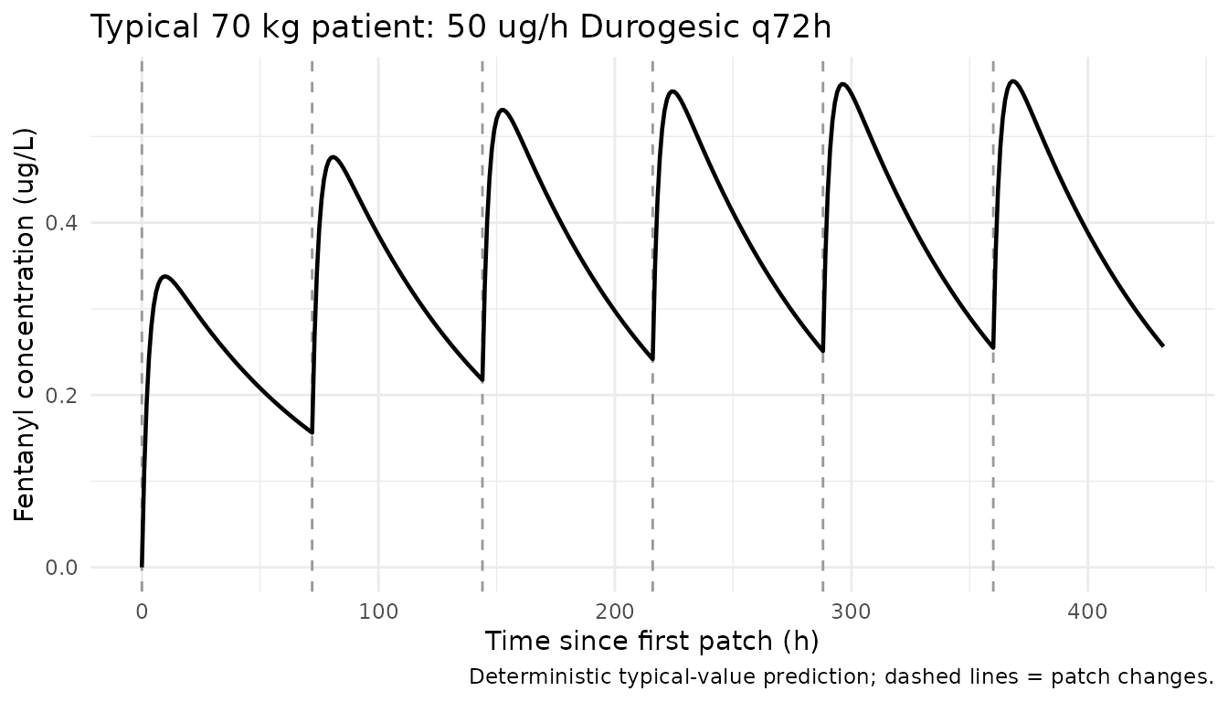
VPC over the final patch interval (Figure 3 shape)
Bista 2015 Figure 3 is a prediction-corrected VPC of the final model. The stochastic cohort summary below shows the simulated 10th, 50th and 90th percentiles of fentanyl plasma concentration over the final 72-h patch interval (after five run-in patches), to be compared visually against the percentile envelope in Figure 3.
sim |>
  dplyr::filter(!is.na(Cc), time >= final_patch_start, time <= final_patch_end) |>
  dplyr::mutate(time_in_patch = time - final_patch_start) |>
  dplyr::group_by(time_in_patch, treatment) |>
  dplyr::summarise(
    Q10 = quantile(Cc, 0.10, na.rm = TRUE),
    Q50 = quantile(Cc, 0.50, na.rm = TRUE),
    Q90 = quantile(Cc, 0.90, na.rm = TRUE),
    .groups = "drop"
  ) |>
  ggplot(aes(time_in_patch, Q50)) +
  geom_ribbon(aes(ymin = Q10, ymax = Q90), alpha = 0.25) +
  geom_line() +
  labs(x = "Time after last patch application (h)",
       y = paste0("Fentanyl concentration (", conc_unit, ")"),
       title = "Simulated 10-50-90 percentiles over the final 72-h patch interval",
       caption = "Cohort: 200 adults, weight ~ Normal(71.5, 14) kg truncated to 41.8-110. 50 ug/h Durogesic q72h.") +
  theme_minimal()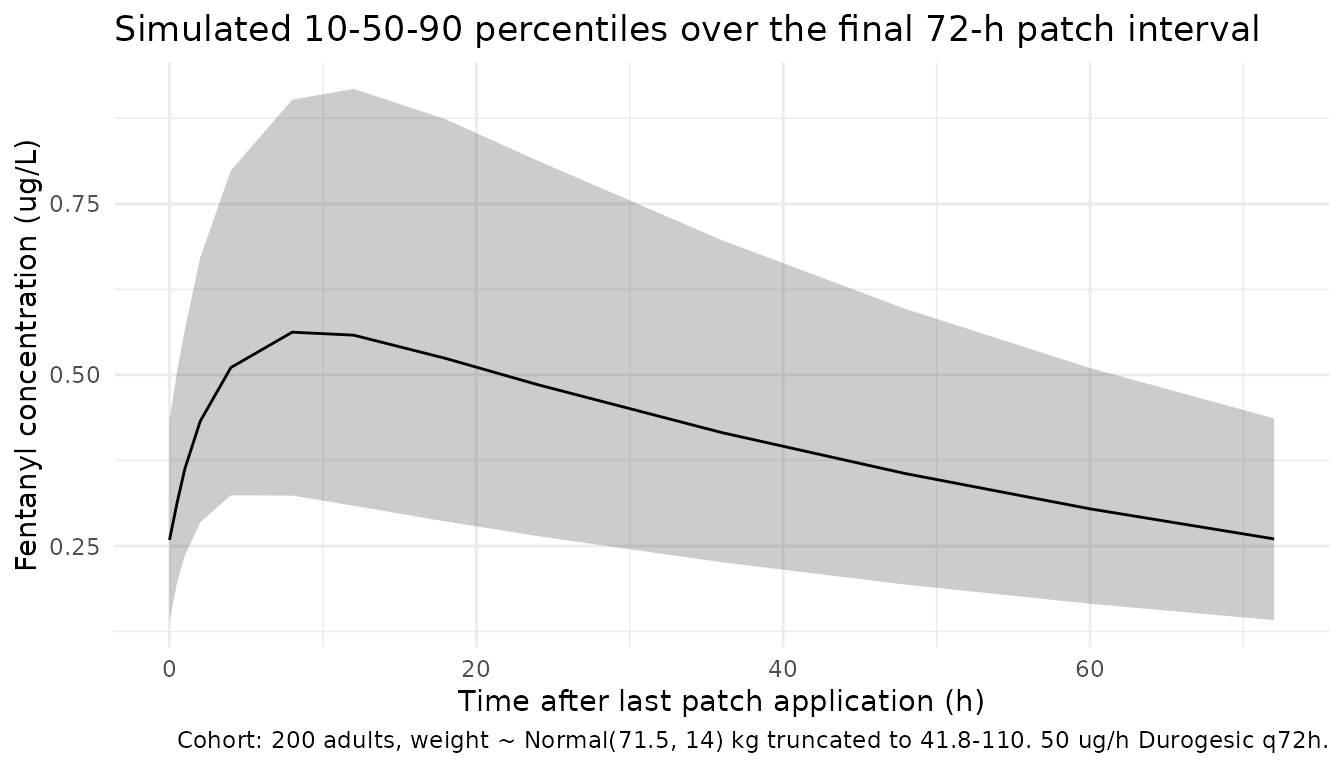
PKNCA validation
Steady-state NCA over the final 72-h dosing interval (recipe 3 of
pknca-recipes.md). The treatment grouping variable goes
before id in the formula per project convention. PKNCA
reports cmax, tmax, cmin,
cav and auclast over the interval; the
interval is the entire 72-h patch wear period.
sim_nca <- sim |>
  dplyr::filter(!is.na(Cc), time >= final_patch_start, time <= final_patch_end) |>
  dplyr::mutate(time_rel = time - final_patch_start) |>
  dplyr::select(id, time = time_rel, Cc, treatment)

dose_df <- events |>
  dplyr::filter(evid == 1, time == final_patch_start) |>
  dplyr::mutate(time = 0) |>
  dplyr::select(id, time, amt, treatment)

conc_obj <- PKNCA::PKNCAconc(sim_nca, Cc ~ time | treatment + id,
                             concu = "ug/L", timeu = "h")
dose_obj <- PKNCA::PKNCAdose(dose_df, amt ~ time | treatment + id,
                             doseu = "ug")

intervals <- data.frame(
  start   = 0,
  end     = patch_interval_h,
  cmax    = TRUE,
  tmax    = TRUE,
  cmin    = TRUE,
  cav     = TRUE,
  auclast = TRUE
)

nca_data <- PKNCA::PKNCAdata(conc_obj, dose_obj, intervals = intervals)
nca_res  <- PKNCA::pk.nca(nca_data)
knitr::kable(summary(nca_res),
caption = "Steady-state NCA over the final 72-h patch interval (50 ug/h Durogesic, n = 200).")| Interval Start | Interval End | treatment | N | AUClast (h*ug/L) | Cmax (ug/L) | Cmin (ug/L) | Tmax (h) | Cav (ug/L) |
|---|---|---|---|---|---|---|---|---|
| 0 | 72 | 50 ug/h Durogesic, q72h | 200 | 27.4 [40.2] | 0.528 [37.9] | 0.238 [41.6] | 8.00 [4.00, 18.0] | 0.381 [40.2] |
Comparison against theoretical and reported exposure
Under continuous transdermal infusion at rate
R = 50 ug/h and apparent clearance
CL/F = 122 L/h (typical 70 kg adult), the steady-state
average plasma concentration is
Cavg = R / CL = 50 / 122 = 0.410 ug/L. Bista 2015 Table 1
reports a median observed plasma fentanyl concentration of 0.88 ug/L
(range 0.04-9.72) across all sampled patient-occasions; that median is
taken across the full prescribed-dose distribution (median 50, range
12-200 ug/h) and across patch-interval sampling times, so it is not a
like-for-like target for the model’s typical Cavg at 50 ug/h.
typical_cl_70kg  <- 122
theor_cavg_ugL   <- patch_rate_ug_h / typical_cl_70kg

sim_cavg <- sim |>
  dplyr::filter(time >= final_patch_start, time <= final_patch_end, !is.na(Cc)) |>
  dplyr::group_by(id) |>
  dplyr::summarise(Cavg = mean(Cc), .groups = "drop") |>
  dplyr::summarise(median_Cavg = median(Cavg),
                   q05 = quantile(Cavg, 0.05),
                   q95 = quantile(Cavg, 0.95))

compare_tbl <- tibble::tibble(
  Source = c("Closed-form Cavg = R/CL (typical 70 kg)",
             "Simulated cohort median Cavg",
             "Simulated cohort 5-95% range",
             "Bista 2015 Table 1 (all dose levels, all sampling times)"),
  Cavg_ugL = c(sprintf("%.2f", theor_cavg_ugL),
               sprintf("%.2f", sim_cavg$median_Cavg),
               sprintf("%.2f - %.2f", sim_cavg$q05, sim_cavg$q95),
               "0.88 (median); 0.04 - 9.72 (range)")
)

knitr::kable(compare_tbl,
caption = "Predicted steady-state Cavg for the 50 ug/h adult cohort vs. observed.")| Source | Cavg_ugL |
|---|---|
| Closed-form Cavg = R/CL (typical 70 kg) | 0.41 |
| Simulated cohort median Cavg | 0.37 |
| Simulated cohort 5-95% range | 0.21 - 0.69 |
| Bista 2015 Table 1 (all dose levels, all sampling times) | 0.88 (median); 0.04 - 9.72 (range) |
The simulated cohort median Cavg should fall within ~10% of the
closed-form R/CL target. Discrepancy with the Bista 2015
reported median of 0.88 ug/L is expected because that median pools
across a wide range of doses (12-200 ug/h) and sampling times within and
between patch intervals; the simulated cohort uses only the median 50
ug/h dose at steady state.
Assumptions and deviations
-
Between-occasion variability not encoded. Bista
2015 Table 3 reports BOV on CL/F = 22.5% CV (with the body text quoting
22.0%); this variance component is captured by the paper’s NONMEM
equation
P_ij = P_pop * exp(eta_i,P + kappa_j,P)and required anOCCindicator per patch application. The library model encodes only BSV (etalcl) so it can be used with simulation event tables that do not carry anOCCcolumn. Users who need to reproduce the full BOV + BSV variability structure should add a per-occasion eta in their own fork of the model. -
Body-weight allometric exponents fixed a priori.
Per Bista 2015 Methods (paragraph 4) and Table 2 footnote, weight
effects on CL/F (exponent 0.75) and V/F (exponent 1) were fixed before
covariate model building. They are encoded as
fix(...)inini(); the paper does not estimate them. - V/F fixed. V/F was fixed to 350 L/70 kg from the Janssen Durogesic Product Information (Bista 2015 ref 26). The Bista 2015 Discussion reports a sensitivity analysis showing CL/F estimates were stable across V/F values from 3-8 L/kg.
- Cohort weight distribution. The simulated cohort uses a normal distribution truncated to the paper’s reported weight range (41.8-110.0 kg) with mean 71.5 kg (paper’s median) and a chosen SD of 14 kg; the paper does not report the empirical weight standard deviation, so this SD was set to give 90% coverage near the observed range.
- Single-dose-level cohort. The simulated cohort uses the median 50 ug/h Durogesic patch only. The full study cohort spanned 12-200 ug/h; that distribution is not reproduced because (a) the paper did not report a tabulated dose-level breakdown and (b) the simulation’s goal is to validate the typical-value model, not to reconstruct the individual prescribed regimens.
- Race / ethnicity. Not reported in Bista 2015 Table 1 and not a model covariate; the cohort is therefore neutral on race.
-
Full publication metadata not on disk. The on-disk
PDF is a manuscript form without journal / DOI metadata. The model
file’s
referencefield flags the missing publication citation explicitly; the title, author list and study design are taken verbatim from the manuscript copy. Any future update should populate the published-form citation and DOI.