Oral vancomycin fecal pharmacokinetics in mice (Maskawa 2025)
Source:vignettes/articles/Maskawa_2025_vancomycin_mouse.Rmd
Maskawa_2025_vancomycin_mouse.RmdModel and source
- Citation: Maskawa R, Takayasu L, Takayasu H, Watanabe K, Takemine S, Kakimoto T, Takeshita K, Narushima S, Suda W, Takayasu M. High-resolution fecal pharmacokinetic modeling in mice with orally administered antibiotics. Sci Rep. 2025;15:24441. doi:10.1038/s41598-025-10293-7.
- Description (main, zero-order gastric emptying, Model 1): Preclinical (mouse). Gastrointestinal transit model for fecal concentrations of orally administered, non-absorbed vancomycin in male C57BL/6N mice (the paper’s zero-order Model 1). The dose empties from the stomach into the cecum at a constant rate over a duration t_in, is eliminated from the cecum by first-order transit (k_e), and the fecal concentration is the cecal amount divided by the mass of cecal contents A. The stomach-to-cecum and cecum-to-feces transit delays are only identifiable as their sum t_tot, which is applied as a lag on the cecal input, so the cecum state holds the cecal amount shifted forward to the time it appears in feces. Doses go into cecum with rate = -2 so that dur(cecum) supplies the emptying duration. Fitted per mouse by penalised least squares; typical values are the arithmetic means over the six treated mice and the between-mouse variances are derived from the reported coefficients of variation.
- Description (supplementary, first-order gastric emptying, Model 2): Preclinical (mouse). Gastrointestinal transit model for fecal concentrations of orally administered, non-absorbed vancomycin in male C57BL/6N mice, with first-order gastric emptying (the paper’s supplementary Model 2, the alternative to the zero-order main model Maskawa_2025_vancomycin_mouse). The dose empties from the stomach into the cecum with rate constant k_a, is eliminated from the cecum by first-order transit (k_e), and the fecal concentration is the cecal amount divided by the mass of cecal contents A. The stomach-to-cecum and cecum-to-feces transit delays are only identifiable as their sum t_tot, applied as a lag on the oral dose into stomach. Fitted per mouse by penalised least squares; typical values are the arithmetic means over the six treated mice and the between-mouse variances are derived from the reported coefficients of variation.
- Article: https://doi.org/10.1038/s41598-025-10293-7 (open access; the Supplementary Information holds Model 2 and Tables S1-S2)
Maskawa et al. sampled feces from mice every 4 hours after a single
oral dose of vancomycin, which is essentially not absorbed from the gut,
and described the fecal concentration-time course with a minimal
gastrointestinal transit model. The stomach is a retention compartment
and the cecum a mixing compartment. In the main model (Model 1) the
stomach empties into the cecum at a constant rate q / t_in
for a duration t_in. The cecum empties into the feces by
first-order transit at rate constant k_e. The fecal
concentration is the cecal amount divided by the mass of cecal contents
A. Two transit delays, stomach to cecum
(dt_SC) and cecum to feces (dt_CF), are
identifiable only as their sum t_tot. Methods Eq. 7 gives
the closed-form fecal concentration:
C(t) = 0                                                     for t - t_tot <= 0
C(t) = q / (t_in A k_e) (1 - exp(-k_e (t - t_tot)))          for 0 < t - t_tot <= t_in
C(t) = q / (t_in A k_e) (exp(-k_e (t - t_tot - t_in))
                         - exp(-k_e (t - t_tot)))            for t - t_tot > t_in
The supplementary Model 2 replaces the zero-order emptying with
first-order emptying at rate constant k_a. The authors
found the two models comparably good, with Model 1 slightly better by
RMSE (Table S2). Both are packaged:
| Model file | Gastric emptying | Source |
|---|---|---|
Maskawa_2025_vancomycin_mouse |
zero-order over t_in
|
Main text, Table 2 |
Maskawa_2025_vancomycin_mouse_firstorder |
first-order at k_a
|
Supplementary Information section 2, Table S1 |
Encoding in rxode2
The model has no plasma compartment. Its observation
Ccecum is the fecal concentration (mg vancomycin per g wet
feces).
-
Model 1. The gastric emptying flux
q / t_inis a zero-order infusion intocecum, so doses go intocecumwithrate = -2anddur(cecum) <- d1suppliest_in.alag(cecum) <- tlagsuppliest_tot. The lag shifts the whole cecal mass curve forward byt_tot, not just by the stomach-to-cecum delay. Thececumstate is therefore the cecal amount at the moment it is expelled, andcecum / v_cecumis exactly the paper’sC(t) = M_b(t - dt_CF) / A. -
Model 2. Doses go into
stomachas a bolus withalag(stomach) <- tlag. The stomach empties first-order intocecum.
Population
Six male, 8-week-old conventional C57BL/6N mice were each given 0.5
mL of vancomycin hydrochloride solution by mouth at 12:00 on day 0.
Three mice (L1-L3) received 1 mg/mL (q = 0.5 mg) and three
(H1-H3) received 20 mg/mL (q = 10 mg). Three water-only
control mice were not part of the model fit. Food and water were
available ad libitum. Feces were collected every 4 h from day -3 to day
3, then less often until day 36. Vancomycin was quantified by
solid-phase extraction and LC-MS/MS and divided by the fecal wet weight
(Methods, “Mice and fecal sample collection” and “Quantification of
antibiotics”; Fig. 1). Body weight was not reported.
The same information is available programmatically via
readModelDb("Maskawa_2025_vancomycin_mouse")()$population.
Source trace
Each mouse was fitted on its own (basinhopping minimisation of a
squared-error loss with a derivative penalty, lambda = 0.9,
Methods Eq. 8). The packaged typical values are the paper’s
Mean (CV%) row over the six mice. The between-mouse
variances are omega^2 = log(1 + CV^2) from the same
row.
| Parameter (model) | Value | Source location |
|---|---|---|
Model 1 ltlag (t_tot) |
log(5.4 h) | Table 2, Mean row |
Model 1 ld1 (t_in) |
log(12 h) | Table 2, Mean row |
Model 1 lkfec (k_e) |
log(0.41 1/h) | Table 2, Mean row |
Model 1 lv_cecum (A) |
log(0.31 g) | Table 2, Mean row |
Model 1 etaltlag, etald1,
etalkfec, etalv_cecum
|
0.2559, 0.3708, 0.2073, 0.3524 | Table 2, CV 54 / 67 / 48 / 65 % |
Model 1 addSd_Ccecum
|
0.21 mg/g | Table S2, Model1 RMSE, column ‘All’ |
Model 2 ltlag (t_tot) |
log(6.7 h) | Table S1, Mean row |
Model 2 lkst (k_a) |
log(0.32 1/h) | Table S1, Mean row |
Model 2 lkfec (k_e) |
log(0.36 1/h) | Table S1, Mean row |
Model 2 lv_cecum (A) |
log(0.40 g) | Table S1, Mean row |
Model 2 etaltlag, etalkst,
etalkfec, etalv_cecum
|
0.1919, 0.2476, 0.2813, 0.6033 | Table S1, CV 46 / 53 / 57 / 91 % |
Model 2 addSd_Ccecum
|
0.60 mg/g | Table S2, Model2 RMSE, column ‘All’ |
Model 1 d/dt(cecum), dur(cecum)
|
n/a | Methods Eq. 2-3 |
Model 2 d/dt(stomach), d/dt(cecum)
|
n/a | Supplementary Information section 2 |
alag() = t_tot = dt_SC + dt_CF
|
n/a | Methods Eq. 6-7; Supplement section 2 |
Ccecum <- cecum / v_cecum |
n/a | Methods Eq. 5-7 |
The per-mouse estimates used below are transcribed from Table 2 (Model 1) and Table S1 (Model 2). The observed NCA values come from Table 1.
mice <- tibble::tribble(
  ~mouse, ~dose_group,      ~q,
  "L1",   "Low (0.5 mg)",   0.5,
  "L2",   "Low (0.5 mg)",   0.5,
  "L3",   "Low (0.5 mg)",   0.5,
  "H1",   "High (10 mg)",   10,
  "H2",   "High (10 mg)",   10,
  "H3",   "High (10 mg)",   10
) |>
  mutate(id = seq_len(n()))

# Table 2: zero-order Model 1
par_m1 <- tibble::tribble(
  ~mouse, ~t_tot, ~t_in, ~k_e, ~A,
  "L1",   4.2,    4.2,   0.35, 0.24,
  "L2",   5.0,    7.0,   0.57, 0.33,
  "L3",   3.2,    7.8,   0.66, 0.17,
  "H1",   12,     23,    0.17, 0.15,
  "H2",   4.0,    25,    0.16, 0.22,
  "H3",   4.3,    7.1,   0.58, 0.74
)

# Table S1: first-order Model 2
par_m2 <- tibble::tribble(
  ~mouse, ~t_tot, ~k_a, ~k_e, ~A,
  "L1",   4.6,    0.42, 0.62, 0.12,
  "L2",   7.7,    0.60, 0.60, 0.26,
  "L3",   3.6,    0.37, 0.37, 0.29,
  "H1",   13,     0.11, 0.11, 0.24,
  "H2",   6.5,    0.12, 0.12, 0.29,
  "H3",   5.0,    0.34, 0.34, 1.2
)

# Table 1: observed (data-derived) fecal NCA. AUC is the trapezoidal area over
# the detection window; k_e is a log-linear regression from t_max to t_elim.
obs_nca <- tibble::tribble(
  ~mouse, ~cmax, ~aucinf.obs, ~lambda.z, ~tmax,
  "L1",   1.0,   5.6,         0.35,      8,
  "L2",   0.39,  2.9,         0.68,      12,
  "L3",   0.53,  4.4,         0.21,      8,
  "H1",   14,    370,         0.16,      36,
  "H2",   11,    250,         0.12,      20,
  "H3",   3.9,   24,          0.11,      8
)

# The per-mouse rows reproduce the printed 'Mean' rows, i.e. the packaged
# typical values, to within the two-significant-figure printing (largest
# gap: t_in, 12.35 printed as 12).
means <- c(
  m1_t_tot = mean(par_m1$t_tot) / 5.4,
  m1_t_in = mean(par_m1$t_in) / 12,
  m1_k_e = mean(par_m1$k_e) / 0.41,
  m1_A = mean(par_m1$A) / 0.31,
  m2_t_tot = mean(par_m2$t_tot) / 6.7,
  m2_k_a = mean(par_m2$k_a) / 0.32,
  m2_k_e = mean(par_m2$k_e) / 0.36,
  m2_A = mean(par_m2$A) / 0.40
)
stopifnot(all(abs(means - 1) < 0.03))
The Table S1 mean of k_a computes to 0.327 1/h, which
the supplement prints as 0.32 (truncation rather than rounding). The
packaged value follows the printed 0.32.
Per-mouse replication (Figure 3b and Supplementary Figure S2b)
Each mouse is simulated with its own Table 2 (Model 1) or Table S1
(Model 2) estimates. Random effects are zeroed and the structural
parameters are overridden through params.
mod1 <- readModelDb("Maskawa_2025_vancomycin_mouse")
mod2 <- readModelDb("Maskawa_2025_vancomycin_mouse_firstorder")
mod1_typ <- rxode2::zeroRe(mod1)
#> ℹ parameter labels from comments will be replaced by 'label()'
mod2_typ <- rxode2::zeroRe(mod2)
#> ℹ parameter labels from comments will be replaced by 'label()'

obs_times <- seq(0, 168, by = 0.25)

# Model 1 doses enter cecum as a zero-order infusion with modelled duration.
make_events <- function(mice, cmt, rate) {
  doses <- mice |>
    transmute(id, time = 0, amt = q, rate = rate, cmt = cmt, evid = 1L)
  obs <- tidyr::crossing(id = mice$id, time = obs_times) |>
    mutate(amt = 0, rate = 0, cmt = "cecum", evid = 0L)
  bind_rows(doses, obs) |>
    left_join(select(mice, id, mouse, dose_group), by = "id") |>
    arrange(id, time, desc(evid))
}
ev1 <- make_events(mice, cmt = "cecum", rate = -2)
ev2 <- make_events(mice, cmt = "stomach", rate = 0)

p1 <- mice |>
  left_join(par_m1, by = "mouse") |>
  transmute(
    id,
    ltlag = log(t_tot), ld1 = log(t_in),
    lkfec = log(k_e), lv_cecum = log(A)
  )
p2 <- mice |>
  left_join(par_m2, by = "mouse") |>
  transmute(
    id,
    ltlag = log(t_tot), lkst = log(k_a),
    lkfec = log(k_e), lv_cecum = log(A)
  )

sim1 <- rxode2::rxSolve(
  mod1_typ,
  events = ev1, params = p1, keep = c("mouse", "dose_group"),
  rtol = 1e-10, atol = 1e-12, maxsteps = 1e6
) |>
  as.data.frame() |>
  mutate(model = "Model 1 (zero-order)")
#> ℹ omega/sigma items treated as zero: 'etaltlag', 'etald1', 'etalkfec', 'etalv_cecum'
#> Warning: multi-subject simulation without without 'omega'
sim2 <- rxode2::rxSolve(
  mod2_typ,
  events = ev2, params = p2, keep = c("mouse", "dose_group"),
  rtol = 1e-10, atol = 1e-12, maxsteps = 1e6
) |>
  as.data.frame() |>
  mutate(model = "Model 2 (first-order)")
#> ℹ omega/sigma items treated as zero: 'etaltlag', 'etalkst', 'etalkfec', 'etalv_cecum'
#> Warning: multi-subject simulation without without 'omega'
sim_ind <- bind_rows(sim1, sim2) |>
  mutate(mouse = factor(mouse, levels = mice$mouse))
sim_ind |>
  filter(time <= 96) |>
  ggplot(aes(time, Ccecum, colour = model)) +
  geom_line() +
  facet_wrap(~mouse, scales = "free_y") +
  labs(
    x = "Time after antibiotic administration (h)",
    y = "Fecal concentration (mg/g)",
    colour = NULL,
    title = "Per-mouse fecal vancomycin profiles",
    caption = paste(
      "Replicates Figure 3b (Model 1) and Supplementary Figure S2b",
      "(Model 2) of Maskawa 2025."
    )
  ) +
  theme(legend.position = "bottom")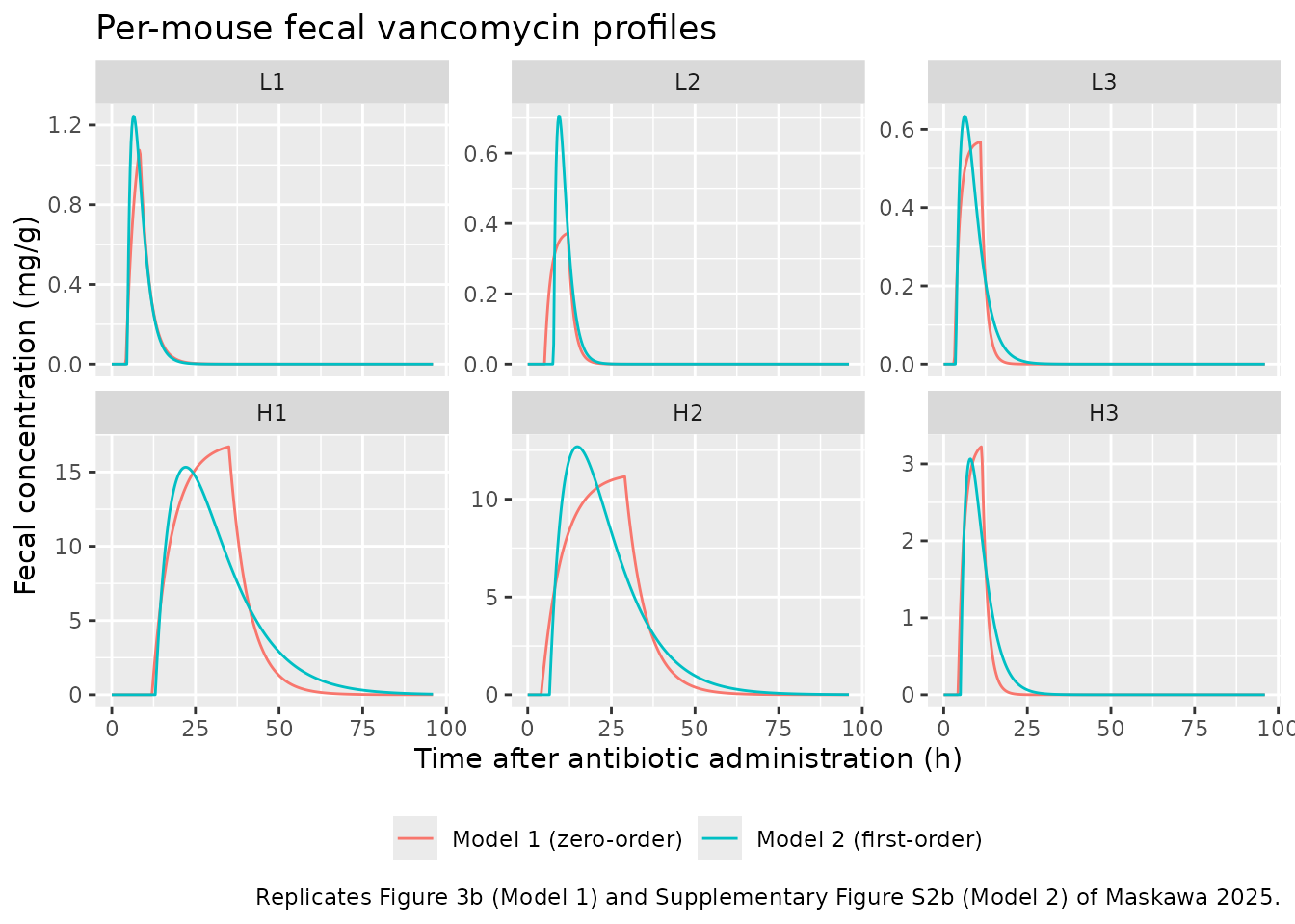
The Model 1 curves reproduce the fitted red curves of Figure 3b. In
Model 1 the peak always falls at the end of gastric emptying,
t = t_tot + t_in. The chunk below compares the simulated
peaks with the peaks of the Figure 3b fitted curves, which the
maintainers read off the published figure.
fig3b_peak <- tibble::tribble(
  ~mouse, ~fig_peak,
  "L1",   1.05,
  "L2",   0.385,
  "L3",   0.55,
  "H1",   17.3,
  "H2",   11.2,
  "H3",   3.25
)
peak_check <- sim1 |>
  group_by(mouse) |>
  summarise(sim_peak = max(Ccecum), t_peak = time[which.max(Ccecum)], .groups = "drop") |>
  left_join(fig3b_peak, by = "mouse") |>
  left_join(par_m1, by = "mouse") |>
  mutate(pct_diff = 100 * (sim_peak / fig_peak - 1))
peak_check |>
  select(mouse, fig_peak, sim_peak, pct_diff, t_peak, t_tot, t_in) |>
  rename(
    "Figure 3b peak (mg/g)" = fig_peak,
    "Simulated peak (mg/g)" = sim_peak,
    "% diff" = pct_diff,
    "Simulated t_max (h)" = t_peak,
    "t_tot (h)" = t_tot,
    "t_in (h)" = t_in
  ) |>
knitr::kable(digits = 3, caption = "Model 1 per-mouse peaks vs. Figure 3b.")| mouse | Figure 3b peak (mg/g) | Simulated peak (mg/g) | % diff | Simulated t_max (h) | t_tot (h) | t_in (h) |
|---|---|---|---|---|---|---|
| H1 | 17.300 | 16.709 | -3.418 | 35.00 | 12.0 | 23.0 |
| H2 | 11.200 | 11.156 | -0.397 | 29.00 | 4.0 | 25.0 |
| H3 | 3.250 | 3.223 | -0.821 | 11.25 | 4.3 | 7.1 |
| L1 | 1.050 | 1.074 | 2.268 | 8.25 | 4.2 | 4.2 |
| L2 | 0.385 | 0.373 | -3.192 | 12.00 | 5.0 | 7.0 |
| L3 | 0.550 | 0.568 | 3.273 | 11.00 | 3.2 | 7.8 |
# Figure reading is good to a few percent; measured |% diff| <= 5%.
stopifnot(
  max(abs(peak_check$pct_diff)) < 10,
  max(abs(peak_check$t_peak - (peak_check$t_tot + peak_check$t_in))) <= 0.25
)
The Model 2 curves are checked the same way against the fitted curves
of Supplementary Figure S2b. In Model 2 the peak falls at
t_tot + log(k_a / k_e) / (k_a - k_e), which is
t_tot + 1 / k when the two constants are equal.
figs2b_peak <- tibble::tribble(
  ~mouse, ~fig_peak,
  "L1",   1.23,
  "L2",   0.72,
  "L3",   0.63,
  "H1",   15.2,
  "H2",   12.7,
  "H3",   3.05
)
peak_check2 <- sim2 |>
  group_by(mouse) |>
  summarise(sim_peak = max(Ccecum), .groups = "drop") |>
  left_join(figs2b_peak, by = "mouse") |>
  mutate(pct_diff = 100 * (sim_peak / fig_peak - 1))
peak_check2 |>
  rename(
    "Figure S2b peak (mg/g)" = fig_peak,
    "Simulated peak (mg/g)" = sim_peak,
    "% diff" = pct_diff
  ) |>
knitr::kable(digits = 3, caption = "Model 2 per-mouse peaks vs. Supplementary Figure S2b.")| mouse | Simulated peak (mg/g) | Figure S2b peak (mg/g) | % diff |
|---|---|---|---|
| H1 | 15.328 | 15.20 | 0.839 |
| H2 | 12.685 | 12.70 | -0.119 |
| H3 | 3.065 | 3.05 | 0.494 |
| L1 | 1.245 | 1.23 | 1.254 |
| L2 | 0.706 | 0.72 | -1.994 |
| L3 | 0.634 | 0.63 | 0.659 |
Check against the closed-form solutions
Methods Eq. 7 gives the Model 1 solution in closed form. The Model 2
solution is the Bateman function shifted by t_tot
(Supplementary Information section 2). In five of the six Table S1 fits
k_a equals k_e, which makes the printed
k_a q / (A (k_e - k_a)) form singular. The comparison
therefore uses its limit, q k t' exp(-k t') / A, when the
two constants are equal.
cf_model1 <- function(t, q, t_tot, t_in, k_e, A) {
  s <- t - t_tot
  amp <- q / (t_in * A * k_e)
  ifelse(
    s <= 0, 0,
    ifelse(
      s <= t_in,
      amp * (1 - exp(-k_e * s)),
      amp * (exp(-k_e * (s - t_in)) - exp(-k_e * s))
    )
  )
}
cf_model2 <- function(t, q, t_tot, k_a, k_e, A) {
  s <- pmax(t - t_tot, 0)
  if (isTRUE(all.equal(k_a, k_e))) {
    q * k_a * s * exp(-k_a * s) / A
  } else {
    k_a * q / (A * (k_e - k_a)) * (exp(-k_a * s) - exp(-k_e * s))
  }
}

cf1 <- sim1 |>
  left_join(par_m1, by = "mouse") |>
  left_join(select(mice, mouse, q), by = "mouse") |>
  group_by(mouse) |>
  mutate(
    cf = cf_model1(time, q[1], t_tot[1], t_in[1], k_e[1], A[1]),
    err = abs(Ccecum - cf) / max(cf)
  ) |>
  summarise(max_rel_err = max(err), .groups = "drop") |>
  mutate(model = "Model 1")
cf2 <- sim2 |>
  left_join(par_m2, by = "mouse") |>
  left_join(select(mice, mouse, q), by = "mouse") |>
  group_by(mouse) |>
  mutate(
    cf = cf_model2(time, q[1], t_tot[1], k_a[1], k_e[1], A[1]),
    err = abs(Ccecum - cf) / max(cf)
  ) |>
  summarise(max_rel_err = max(err), .groups = "drop") |>
  mutate(model = "Model 2")
cf_tab <- bind_rows(cf1, cf2)
knitr::kable(
  cf_tab |> select(model, mouse, max_rel_err),
  digits = 12,
  caption = paste(
    "Largest ODE vs closed-form difference, relative to the",
    "mouse's peak concentration."
  )
)| model | mouse | max_rel_err |
|---|---|---|
| Model 1 | H1 | 2.4e-11 |
| Model 1 | H2 | 1.7e-11 |
| Model 1 | H3 | 5.2e-11 |
| Model 1 | L1 | 5.5e-11 |
| Model 1 | L2 | 9.0e-11 |
| Model 1 | L3 | 7.0e-11 |
| Model 2 | H1 | 6.0e-12 |
| Model 2 | H2 | 6.0e-12 |
| Model 2 | H3 | 6.4e-11 |
| Model 2 | L1 | 7.1e-11 |
| Model 2 | L2 | 4.3e-11 |
| Model 2 | L3 | 3.0e-11 |
Mass balance: AUC = q / (A k_e)
Vancomycin is not absorbed, so the whole dose leaves through the
cecum. The area under the fecal concentration curve is therefore
q / (A k_e) in both models. PKNCA on the per-mouse
simulations recovers it.
nca_input <- function(sim) {
  # Floor the integrator's sub-atol undershoot and drop the numerically-zero
  # tail after the peak so that lambda.z follows the true terminal slope.
  stopifnot(all(sim$Ccecum >= -1e-6 * max(sim$Ccecum, na.rm = TRUE), na.rm = TRUE))
  sim |>
    filter(!is.na(Ccecum)) |>
    mutate(Ccecum = pmax(Ccecum, 0)) |>
    group_by(mouse) |>
    filter(time <= time[which.max(Ccecum)] | Ccecum >= 1e-6 * max(Ccecum)) |>
    ungroup() |>
    select(mouse, dose_group, time, Ccecum) |>
    mutate(mouse = as.character(mouse))
}
run_nca <- function(sim, events) {
  conc <- nca_input(sim)
  dose <- events |>
    filter(evid == 1) |>
    select(mouse, dose_group, time, amt)
  dat <- PKNCA::PKNCAdata(
    PKNCA::PKNCAconc(conc, Ccecum ~ time | dose_group + mouse),
    PKNCA::PKNCAdose(dose, amt ~ time | dose_group + mouse),
    intervals = data.frame(
      start = 0, end = Inf,
      cmax = TRUE, tmax = TRUE, aucinf.obs = TRUE, lambda.z = TRUE
    )
  )
  PKNCA::pk.nca(dat)
}
nca1 <- run_nca(sim1, ev1)
nca2 <- run_nca(sim2, ev2)

auc_check <- bind_rows(
  as.data.frame(nca1) |> mutate(model = "Model 1"),
  as.data.frame(nca2) |> mutate(model = "Model 2")
) |>
  filter(PPTESTCD == "aucinf.obs") |>
  left_join(
    bind_rows(
      par_m1 |> mutate(model = "Model 1"),
      par_m2 |> mutate(model = "Model 2")
    ),
    by = c("model", "mouse")
  ) |>
  left_join(select(mice, mouse, q), by = "mouse") |>
  mutate(
    auc_theory = q / (A * k_e),
    pct_diff = 100 * (PPORRES / auc_theory - 1)
  )
auc_check |>
  select(model, mouse, PPORRES, auc_theory, pct_diff) |>
  rename(
    "PKNCA AUCinf (mg*h/g)" = PPORRES,
    "q / (A k_e) (mg*h/g)" = auc_theory,
    "% diff" = pct_diff
  ) |>
knitr::kable(digits = 3, caption = "Mass-balance check of the fecal AUC.")| model | mouse | PKNCA AUCinf (mg*h/g) | q / (A k_e) (mg*h/g) | % diff |
|---|---|---|---|---|
| Model 1 | H1 | 392.142 | 392.157 | -0.004 |
| Model 1 | H2 | 284.082 | 284.091 | -0.003 |
| Model 1 | H3 | 23.285 | 23.299 | -0.062 |
| Model 1 | L1 | 5.949 | 5.952 | -0.053 |
| Model 1 | L2 | 2.657 | 2.658 | -0.042 |
| Model 1 | L3 | 4.456 | 4.456 | -0.001 |
| Model 2 | H1 | 378.759 | 378.788 | -0.008 |
| Model 2 | H2 | 287.330 | 287.356 | -0.009 |
| Model 2 | H3 | 24.492 | 24.510 | -0.073 |
| Model 2 | L1 | 6.722 | 6.720 | 0.029 |
| Model 2 | L2 | 3.204 | 3.205 | -0.043 |
| Model 2 | L3 | 4.661 | 4.660 | 0.015 |
Comparison against the observed NCA (Table 1)
Table 1 holds NCA values computed by the authors from the measured fecal data. The simulations use each mouse’s fitted parameters, so the comparison shows how closely each individual fit reproduces its own data. It is not an independent prediction.
nca_units <- c(
  cmax = "mg/g", tmax = "h", aucinf.obs = "mg*h/g", lambda.z = "1/h"
)
cmp1 <- nlmixr2lib::ncaComparisonTable(
  simulated = nca1,
  reference = obs_nca,
  by = "mouse",
  units = nca_units,
  tolerance_pct = 20
)
knitr::kable(
  cmp1,
  caption = paste(
    "Model 1 (Table 2 per-mouse fits) vs. observed Table 1 NCA.",
    "* differs from the reference by >20%."
  )
)| NCA parameter | mouse | Reference | Simulated | % diff |
|---|---|---|---|---|
| Cmax (mg/g) | L1 | 1 | 1.07 | +7.4% |
| Cmax (mg/g) | L2 | 0.39 | 0.373 | -4.4% |
| Cmax (mg/g) | L3 | 0.53 | 0.568 | +7.2% |
| Cmax (mg/g) | H1 | 14 | 16.7 | +19.3% |
| Cmax (mg/g) | H2 | 11 | 11.2 | +1.4% |
| Cmax (mg/g) | H3 | 3.9 | 3.22 | -17.4% |
| Tmax (h) | L1 | 8 | 8.25 | +3.1% |
| Tmax (h) | L2 | 12 | 12 | +0.0% |
| Tmax (h) | L3 | 8 | 11 | +37.5%* |
| Tmax (h) | H1 | 36 | 35 | -2.8% |
| Tmax (h) | H2 | 20 | 29 | +45.0%* |
| Tmax (h) | H3 | 8 | 11.2 | +40.6%* |
| AUC0-∞ (obs) (mg*h/g) | L1 | 5.6 | 5.95 | +6.2% |
| AUC0-∞ (obs) (mg*h/g) | L2 | 2.9 | 2.66 | -8.4% |
| AUC0-∞ (obs) (mg*h/g) | L3 | 4.4 | 4.46 | +1.3% |
| AUC0-∞ (obs) (mg*h/g) | H1 | 370 | 392 | +6.0% |
| AUC0-∞ (obs) (mg*h/g) | H2 | 250 | 284 | +13.6% |
| AUC0-∞ (obs) (mg*h/g) | H3 | 24 | 23.3 | -3.0% |
| λz (1/h) | L1 | 0.35 | 0.35 | -0.0% |
| λz (1/h) | L2 | 0.68 | 0.57 | -16.2% |
| λz (1/h) | L3 | 0.21 | 0.66 | +214.3%* |
| λz (1/h) | H1 | 0.16 | 0.17 | +6.3% |
| λz (1/h) | H2 | 0.12 | 0.16 | +33.3%* |
| λz (1/h) | H3 | 0.11 | 0.58 | +427.3%* |
cmp2 <- nlmixr2lib::ncaComparisonTable(
  simulated = nca2,
  reference = obs_nca,
  by = "mouse",
  units = nca_units,
  tolerance_pct = 20
)
knitr::kable(
  cmp2,
  caption = paste(
    "Model 2 (Table S1 per-mouse fits) vs. observed Table 1 NCA.",
    "* differs from the reference by >20%."
  )
)| NCA parameter | mouse | Reference | Simulated | % diff |
|---|---|---|---|---|
| Cmax (mg/g) | L1 | 1 | 1.25 | +24.5%* |
| Cmax (mg/g) | L2 | 0.39 | 0.706 | +80.9%* |
| Cmax (mg/g) | L3 | 0.53 | 0.634 | +19.7% |
| Cmax (mg/g) | H1 | 14 | 15.3 | +9.5% |
| Cmax (mg/g) | H2 | 11 | 12.7 | +15.3% |
| Cmax (mg/g) | H3 | 3.9 | 3.07 | -21.4%* |
| Tmax (h) | L1 | 8 | 6.5 | -18.8% |
| Tmax (h) | L2 | 12 | 9.25 | -22.9%* |
| Tmax (h) | L3 | 8 | 6.25 | -21.9%* |
| Tmax (h) | H1 | 36 | 22 | -38.9%* |
| Tmax (h) | H2 | 20 | 14.8 | -26.2%* |
| Tmax (h) | H3 | 8 | 8 | +0.0% |
| AUC0-∞ (obs) (mg*h/g) | L1 | 5.6 | 6.72 | +20.0%* |
| AUC0-∞ (obs) (mg*h/g) | L2 | 2.9 | 3.2 | +10.5% |
| AUC0-∞ (obs) (mg*h/g) | L3 | 4.4 | 4.66 | +5.9% |
| AUC0-∞ (obs) (mg*h/g) | H1 | 370 | 379 | +2.4% |
| AUC0-∞ (obs) (mg*h/g) | H2 | 250 | 287 | +14.9% |
| AUC0-∞ (obs) (mg*h/g) | H3 | 24 | 24.5 | +2.0% |
| λz (1/h) | L1 | 0.35 | 0.414 | +18.4% |
| λz (1/h) | L2 | 0.68 | 0.551 | -19.0% |
| λz (1/h) | L3 | 0.21 | 0.34 | +61.7%* |
| λz (1/h) | H1 | 0.16 | 0.101 | -37.1%* |
| λz (1/h) | H2 | 0.12 | 0.11 | -8.2% |
| λz (1/h) | H3 | 0.11 | 0.312 | +183.7%* |
auc_vs_obs <- auc_check |>
  left_join(select(obs_nca, mouse, auc_obs = aucinf.obs), by = "mouse") |>
  mutate(pct_obs = 100 * (PPORRES / auc_obs - 1))
# Deterministic per-mouse solves: measured |% diff| is at most 14% (Model 1,
# H2) and 20% (Model 2, L1). A wrong dose, A or k_e shifts AUC by far more.
stopifnot(
  max(abs(auc_vs_obs$pct_obs[auc_vs_obs$model == "Model 1"])) < 18,
  max(abs(auc_vs_obs$pct_obs[auc_vs_obs$model == "Model 2"])) < 25
)
Reading the starred rows:
- AUC agrees to within about 15% for Model 1 and 20% for Model 2. The largest Model 1 difference is H2 (+14%), where the fitted plateau sits slightly above the 20-28 h observations (Figure 3b).
-
C_max agrees to within 20% for every mouse under
Model 1. H1 is highest (+19%) because the long zero-order emptying
(
t_in= 23 h) builds a plateau above the scattered high-dose samples. H3 is low (-17%) against the Table 1 value of 3.9 mg/g. Figures 2 and 3b, however, show the highest H3 sample at about 2.9 mg/g, so Table 1 probably misprints it. Against 2.9 the model is 11% high. -
t_max in Table 1 is the time of the highest
observed sample, on a 4-h grid. The Model 1 peak is at
t_tot + t_in, which usually falls between samples. For L3, H2 and H3 it falls after the sample that happened to be highest. - Model 2 reproduces AUC equally well but is a looser fit for the peak. It overshoots C_max for L1 and L2 and puts t_max earlier for most mice. This matches Table S2, where Model 2’s RMSE is higher than Model 1’s for every mouse except L1.
-
lambda.z (the Table 1
k_ecolumn) is not expected to match. The paper notes that its Table 1k_ecomes from a log-linear regression betweent_maxandt_elim. The modelk_ecomes from fitting on the original scale, and the two “differ from those listed in Table 1” (Results, “Gastrointestinal transit model”). The simulated terminal slope equals the modelk_e, by construction.
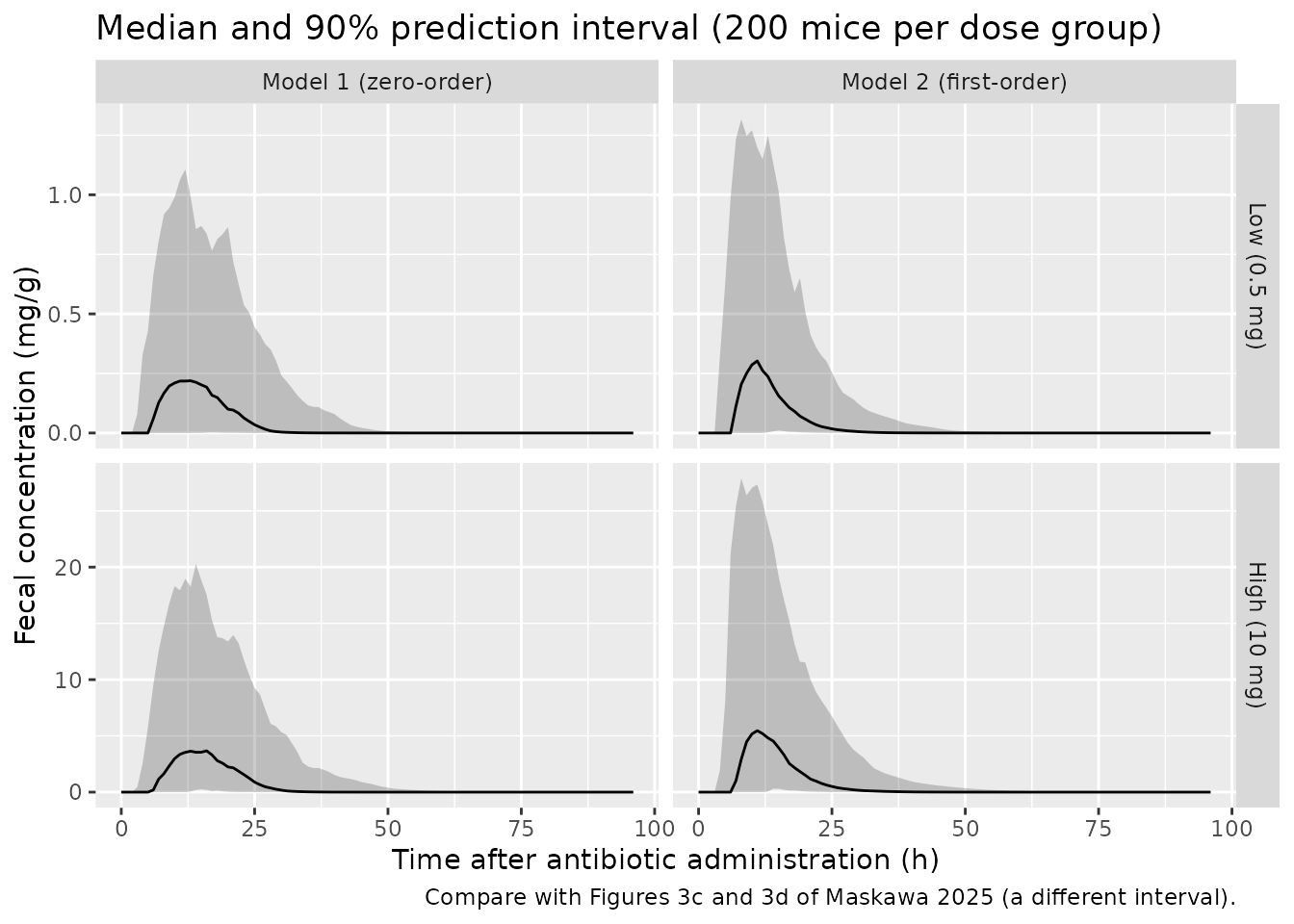
Between-mouse variability (Figures 3c and 3d)
Figures 3c and 3d show bootstrap confidence bands, built by refitting pooled-by-dose-group data on 80% of the time points. That procedure cannot be rerun without the data. The chunk below shows instead what the packaged between-mouse variability implies: 200 virtual mice per dose group, with the 90% prediction interval of the individual fecal concentration. Residual error is excluded.
set.seed(2025)
rxode2::rxSetSeed(2025)
n_per_arm <- 200
vpc_times <- seq(0, 96, by = 1)
make_vpc_events <- function(cmt, rate) {
  bind_rows(
    tibble(dose_group = "Low (0.5 mg)", q = 0.5, id = seq_len(n_per_arm)),
    tibble(dose_group = "High (10 mg)", q = 10, id = n_per_arm + seq_len(n_per_arm))
  ) |>
    (\(d) {
      bind_rows(
        d |> transmute(id, dose_group, time = 0, amt = q, rate = rate, cmt = cmt, evid = 1L),
        tidyr::crossing(d |> select(id, dose_group), time = vpc_times) |>
          mutate(amt = 0, rate = 0, cmt = "cecum", evid = 0L)
      )
    })() |>
    arrange(id, time, desc(evid))
}
ev_vpc1 <- make_vpc_events("cecum", -2)
ev_vpc2 <- make_vpc_events("stomach", 0)
stopifnot(!anyDuplicated(unique(ev_vpc1[, c("id", "time", "evid")])))

vpc <- bind_rows(
  rxode2::rxSolve(mod1, events = ev_vpc1, keep = "dose_group") |>
    as.data.frame() |>
    mutate(model = "Model 1 (zero-order)"),
  rxode2::rxSolve(mod2, events = ev_vpc2, keep = "dose_group") |>
    as.data.frame() |>
    mutate(model = "Model 2 (first-order)")
) |>
  mutate(dose_group = factor(dose_group, levels = c("Low (0.5 mg)", "High (10 mg)")))
#> ℹ parameter labels from comments will be replaced by 'label()'
#> ℹ parameter labels from comments will be replaced by 'label()'

vpc |>
  group_by(model, dose_group, time) |>
  summarise(
    Q05 = quantile(Ccecum, 0.05),
    Q50 = quantile(Ccecum, 0.50),
    Q95 = quantile(Ccecum, 0.95),
    .groups = "drop"
  ) |>
  ggplot(aes(time, Q50)) +
  geom_ribbon(aes(ymin = Q05, ymax = Q95), alpha = 0.25) +
  geom_line() +
  facet_grid(dose_group ~ model, scales = "free_y") +
  labs(
    x = "Time after antibiotic administration (h)",
    y = "Fecal concentration (mg/g)",
    title = "Median and 90% prediction interval (200 mice per dose group)",
    caption = "Compare with Figures 3c and 3d of Maskawa 2025 (a different interval)."
  )
# Dose linearity: with no dose effect in the model, the dose-normalised
# median peak is the same in both arms up to Monte-Carlo error.
peaks <- vpc |>
  filter(model == "Model 1 (zero-order)") |>
  group_by(dose_group, id) |>
  summarise(cmax = max(Ccecum), .groups = "drop") |>
  mutate(cmax_dn = cmax / ifelse(dose_group == "High (10 mg)", 10, 0.5)) |>
  group_by(dose_group) |>
  summarise(med = median(cmax_dn), .groups = "drop")
ratio <- peaks$med[peaks$dose_group == "High (10 mg)"] /
  peaks$med[peaks$dose_group == "Low (0.5 mg)"]
# Median of 200 draws: about 6% Monte-Carlo SE per arm, so the ratio sits
# within 0.75-1.33 with wide margin; a dose mis-scaling gives 20x or 0.05x.
stopifnot(ratio > 0.75, ratio < 1.33)
Assumptions and deviations
-
Typical values are arithmetic means of individual
fits. The authors fitted each mouse separately and did not fit
a population model. The packaged typical values are the paper’s
Mean (CV%)rows in Table 2 and Table S1. The log-normal between-mouse variances are derived from those CVs aslog(1 + CV^2). That means the typical value sits near the mean, not the median, of the log-normal distribution. The CVs pool both dose groups, so they include the longer emptying (t_in) and slower cecal transit (k_e) seen in two of the three high-dose mice. The paper treats this as a possible dose-dependent change in gastrointestinal motility that it could not establish with three mice per group. The model carries no dose effect. - Residual error. The loss function is unweighted squared error plus a derivative penalty (Methods Eq. 8), so the residual error is additive. Its SD is the pooled RMSE across the six mice (Table S2, column ‘All’: 0.21 mg/g for Model 1 and 0.60 mg/g for Model 2). The pooled RMSE is dominated by the high-dose mice. The per-mouse RMSE of the low-dose fits is about 0.004-0.016 mg/g, so simulating low-dose observations with the pooled SD overstates their noise.
-
Transit delays. Only
t_tot = dt_SC + dt_CFis identifiable and reported. The model applies it as a single lag on the cecal (Model 1) or gastric (Model 2) input. The paper’s Model 1 stomach massM_a(t) = q (1 - t / t_in)is not carried as a state, because the zero-order infusion reproduces its outflow exactly. Doses intocecummust userate = -2fordur(cecum)to take effect. -
Minor text-table differences. The Results text
gives the low-dose
t_inrange as 4.1-7.8 h and the H3 cecal content mass as 0.76 g. Table 2 lists L1t_in= 4.2 h and H3A= 0.74 g. The table values are used here. The Table 2 means are the same either way. Table 1 lists the H3 observed C_max as 3.9 mg/g, but the highest H3 sample in Figures 2 and 3b is about 2.9 mg/g. The comparison table keeps the printed 3.9. The observed NCA values are used only for comparison, not in the model. -
Units. Doses are in mg (0.5 mL of 1 or 20 mg/mL),
Ais in g of cecal contents, and concentrations are mg per g of wet feces, as in Table 1 and Figure 3. - Figure-derived values. The peak concentrations of the fitted curves in Figure 3b and Supplementary Figure S2b, used in the per-mouse peak checks, were read off the published figures by the maintainers, to about +/-3%. They are used only for validation; every model parameter comes from Table 2, Table S1 or Table S2.
- No erratum or correction notice was found for this article as of 2026-11-05.