Midomafetamine (MDMA) and MDA (Huestis 2025)
Source:vignettes/articles/Huestis_2025_midomafetamine.Rmd
Huestis_2025_midomafetamine.RmdModel and source
- Citation: Huestis MA, Smith WB, Leonowens C, Blanchard R, Viaccoz A, Spargo E, Miner NB, Yazar-Klosinski B. MDMA pharmacokinetics: A population and physiologically based pharmacokinetics model-informed analysis. CPT Pharmacometrics Syst Pharmacol. 2025;14(2):376-388. doi:10.1002/psp4.13282. Only the population PK model (Table 2) is encoded; the paper’s Simcyp minimal-PBPK model with CYP2D6 mechanism-based inhibition is not.
- Description: One-compartment oral population PK model for midomafetamine (MDMA) with an absorption lag followed by sequential zero-order then first-order absorption, linked to a two-compartment model of its metabolite tenamfetamine (MDA, 3,4-methylenedioxyamphetamine) formed from a fixed 10% of MDMA clearance, with body-weight effects on MDMA CL/F and V/F and on MDA CL and Q, a sex effect on MDA peripheral volume, high-fat-meal and fasted effects on MDMA ka, and an empirical study effect on MDMA CL/F and V/F, in healthy adult volunteers (Huestis 2025)
- Article: https://doi.org/10.1002/psp4.13282 (open access; Supplementary Materials Data S1 hold the study designs, Table S1 covariate list, Table S4 demographics and the PBPK input and output tables)
Huestis 2025 reports two models for midomafetamine (3,4-methylenedioxymethamphetamine, MDMA): a NONMEM population PK model of MDMA and its active metabolite 3,4-methylenedioxyamphetamine (MDA, INN tenamfetamine), and a Simcyp minimal-PBPK model with CYP2D6 mechanism-based inhibition used for split-dose and drug-drug interaction simulations. Only the population PK model is packaged here (see Assumptions and deviations for why the PBPK model is not).
The MDMA model is one-compartment with an absorption lag, a zero-order input of duration D1 into the depot and first-order absorption from it, and linear elimination. A fixed 10% of MDMA clearance forms MDA, which is described by a two-compartment model. MDA was fitted sequentially on the individual MDMA post hoc estimates; the packaged model links the two so both analytes are simulated together.
Population
Huestis 2025 pooled two phase I crossover studies in healthy volunteers (Supplementary Materials; Table S4):
- MPKF (N = 16): open-label randomised-sequence two-period food-effect study; 120 mg MDMA HCl taken after at least 10 h fasting or after a high-fat, high-calorie meal (~800-1000 kcal, ~50% of calories from fat); sampling to 72 h. Median age 40.4 years, median weight 76.3 kg, 50% female, 87.5% White.
- NIDA (N = 49): double-blind placebo-controlled within-subject study; 1.0 and 1.6 mg/kg MDMA HCl (43-150 mg) after a light meal; sampling to 167 h. Median age 23.0 years, median weight 72.6 kg, 34.7% female, 73.5% Black.
Overall: 65 adults aged 18.0-60.1 years (median 25.0), 43.1-113.1 kg (median 73.8), 38.5% female, 40.0% White and 58.5% Black or African American; 2012 MDMA and 1871 MDA plasma concentrations.
The same information is available programmatically via
readModelDb("Huestis_2025_midomafetamine")()$population.
Source trace
Every value is from Huestis 2025 Table 2 unless stated. IIV is printed as %CV = sqrt(omega^2) x 100 (Methods, under Equation 1), so omega^2 = (CV/100)^2; the correlations printed beneath Table 2 give the covariances.
| Equation / parameter | Value | Source location |
|---|---|---|
lcl (MDMA CL/F, 70 kg, NIDA) |
log(41.5 L/h) | Table 2 ‘CL/F’ |
lvc (MDMA V2/F, 70 kg, NIDA) |
log(462 L) | Table 2 ‘V2/F’ |
lka (light breakfast) |
log(1.17 1/h) | Table 2 ‘ka’ |
ltlag |
log(0.322 h) | Table 2 ‘ALAG1’ |
ld1 |
log(0.304 h) | Table 2 ‘D1’ |
e_wt_cl, e_wt_vc
|
1.03, 0.885 | Table 2 ‘Body weight effect on CL/F’, ‘… on V2/F’; Equation 3 |
e_study_mpkf_cl, e_study_mpkf_vc
|
-0.36, -0.263 | Table 2 ‘Study effect on CL/F’, ‘… on V2/F’; Equation 4 |
e_fed_highfat_ka |
-0.484 | Table 2 ‘Fed status effect on ka’; Equation 4 |
e_fasted_ka |
1.93 | Table 2 ‘Fasted status effect on ka’; Equation 4 |
fm |
0.1 (fixed) | Table 2 ‘fmet’ |
lcl_tenamfetamine (MDA CLM, 70 kg) |
log(34.9 L/h) | Table 2 ‘CLM’ |
lvc_tenamfetamine (MDA V3) |
log(20.8 L) | Table 2 ‘V3’ |
lq_tenamfetamine (MDA QM, 70 kg) |
log(79.6 L/h) | Table 2 ‘QM’ |
lvp_tenamfetamine (MDA V4, male) |
log(213 L) | Table 2 ‘V4’ |
e_wt_cl_tenamfetamine,
e_wt_q_tenamfetamine
|
0.580, 1.00 | Table 2 ‘Body weight effect on CLM’, ‘… on QM’ |
e_sexf_vp_tenamfetamine |
-0.181 | Table 2 ‘Sex effect on V4’ |
etalcl, etalvc block |
0.305^2, 0.67 x 0.305 x 0.199, 0.199^2 | Table 2 IIV 30.5% / 19.9%; r = 0.67 |
etalka, etald1
|
0.602^2, 1.53^2 | Table 2 IIV 60.2%, 153% |
| MDA IIV block (CLM, QM, V4) | 0.320, 0.468, 0.352 SD; r = 0.82, 0.86, 0.70 | Table 2 and correlations beneath it |
propSd, addSd,
addSd_mpkf
|
0.207, 8.11 ng/mL, 2.5 ng/mL (fixed) | Table 2 MDMA ‘Prop. Error’, ‘Add. Error NIDA’, ‘Add. Error MPKF’ |
propSd_tenamfetamine,
addSd_tenamfetamine
|
0.122, 0.776 ng/mL | Table 2 MDA ‘Prop. Error’, ‘Add. Error’ |
Residual model Y = C(1 + eps1) + eps2
|
n/a | Equation 2 |
Covariate forms (WT/70)^theta,
(1 + theta X)
|
n/a | Equations 3 and 4; 70 kg reference (Methods; Figure 2 reference individual) |
| Lag, zero-order then first-order absorption | n/a | Methods ‘Model development’ (sequential zero- then first-order); Discussion |
MDA formation fm * CL/F / V2/F * A_central
|
n/a | Results ‘PopPK model analysis’; Table 2 ‘fmet’ |
Typical-value covariate effects (Figure 2)
Figure 2 of Huestis 2025 summarises the covariate effects as the fold-change in AUC0-44 and Cmax relative to a reference individual: a 70-kg White male from the NIDA study, 25 years old, fed a light meal. The model ratios do not depend on the dose, so a single 120 mg dose is used.
mod <- readModelDb("Huestis_2025_midomafetamine")
mod_typ <- rxode2::zeroRe(rxode2::rxode2(mod))
#> ℹ parameter labels from comments will be replaced by 'label()'

scenarios <- tibble::tribble(
  ~scenario,                          ~WT,   ~SEXF, ~STUDY_MPKF, ~FED, ~FED_HIGHFAT,
  "Reference",                        70,    0,     0,           1,    0,
  "Body weight 5th pct (52.06 kg)",   52.06, 0,     0,           1,    0,
  "Body weight 95th pct (96.69 kg)",  96.69, 0,     0,           1,    0,
  "Female vs male",                   70,    1,     0,           1,    0,
  "MPKF vs NIDA",                     70,    0,     1,           1,    0,
  "High-fat meal vs light breakfast", 70,    0,     0,           1,    1,
  "Fasted vs light breakfast",        70,    0,     0,           0,    0
) |>
  mutate(id = row_number())

forest_events <- bind_rows(
  scenarios |> mutate(time = 0, amt = 120, evid = 1L, rate = -2, cmt = "depot", dvid = NA_integer_),
  tidyr::expand_grid(scenarios, time = seq(0, 44, by = 0.01)) |>
    mutate(amt = 0, evid = 0L, rate = 0, cmt = "central", dvid = 1L)
) |>
  arrange(id, time, desc(evid))

forest_sim <- rxode2::rxSolve(mod_typ, forest_events, keep = "scenario", returnType = "data.frame")
#> ℹ omega/sigma items treated as zero: 'etalcl', 'etalvc', 'etalka', 'etald1', 'etalcl_tenamfetamine', 'etalq_tenamfetamine', 'etalvp_tenamfetamine'
#> Warning: multi-subject simulation without without 'omega'

trap <- function(t, y) sum(diff(t) * (head(y, -1) + tail(y, -1)) / 2)
forest_exp <- forest_sim |>
  group_by(scenario) |>
  summarise(
    MDMA_AUC = trap(time, Cc), MDMA_Cmax = max(Cc),
    MDA_AUC = trap(time, Cc_tenamfetamine), MDA_Cmax = max(Cc_tenamfetamine),
    .groups = "drop"
  )
forest_ref <- forest_exp |> filter(scenario == "Reference")
forest_ratio <- forest_exp |>
  filter(scenario != "Reference") |>
  mutate(across(-scenario, ~ .x / forest_ref[[cur_column()]])) |>
  pivot_longer(-scenario, names_to = c("analyte", "metric"), names_sep = "_", values_to = "simulated")
# Huestis 2025 Figure 2 boxes: median [95% CI]. The MDMA panel's middle row is
# labelled 'Sex' but its category is 'MPKF:NIDA', i.e. it is the study effect;
# sex was not retained in the MDMA model.
forest_pub <- tibble::tribble(
  ~scenario,                          ~analyte, ~metric, ~published, ~lo,  ~hi,
  "Body weight 5th pct (52.06 kg)",   "MDMA",   "AUC",   1.3,        1.3,  1.4,
  "Body weight 5th pct (52.06 kg)",   "MDMA",   "Cmax",  1.3,        1.3,  1.3,
  "Body weight 95th pct (96.69 kg)",  "MDMA",   "AUC",   0.72,       0.70, 0.76,
  "Body weight 95th pct (96.69 kg)",  "MDMA",   "Cmax",  0.75,       0.71, 0.78,
  "MPKF vs NIDA",                     "MDMA",   "AUC",   1.5,        1.5,  1.6,
  "MPKF vs NIDA",                     "MDMA",   "Cmax",  1.4,        1.4,  1.4,
  "High-fat meal vs light breakfast", "MDMA",   "AUC",   1.0,        1.0,  1.0,
  "High-fat meal vs light breakfast", "MDMA",   "Cmax",  0.87,       0.86, 0.89,
  "Fasted vs light breakfast",        "MDMA",   "AUC",   1.0,        1.0,  1.0,
  "Fasted vs light breakfast",        "MDMA",   "Cmax",  1.1,        1.1,  1.1,
  "Body weight 5th pct (52.06 kg)",   "MDA",    "AUC",   1.1,        1.1,  1.2,
  "Body weight 5th pct (52.06 kg)",   "MDA",    "Cmax",  1.1,        1.1,  1.1,
  "Body weight 95th pct (96.69 kg)",  "MDA",    "AUC",   0.85,       0.81, 0.90,
  "Body weight 95th pct (96.69 kg)",  "MDA",    "Cmax",  0.93,       0.89, 0.96,
  "Female vs male",                   "MDA",    "AUC",   1.0,        1.0,  1.0,
  "Female vs male",                   "MDA",    "Cmax",  1.1,        1.1,  1.1,
  "MPKF vs NIDA",                     "MDA",    "AUC",   0.97,       0.97, 0.97,
  "MPKF vs NIDA",                     "MDA",    "Cmax",  0.92,       0.91, 0.92,
  "High-fat meal vs light breakfast", "MDA",    "AUC",   0.99,       0.99, 0.99,
  "High-fat meal vs light breakfast", "MDA",    "Cmax",  0.98,       0.98, 0.98,
  "Fasted vs light breakfast",        "MDA",    "AUC",   1.0,        1.0,  1.0,
  "Fasted vs light breakfast",        "MDA",    "Cmax",  1.0,        1.0,  1.0
)

forest_cmp <- forest_pub |>
  inner_join(forest_ratio, by = c("scenario", "analyte", "metric"))
stopifnot(nrow(forest_cmp) == nrow(forest_pub))

# Deterministic typical-value solve against the paper's own boxes. The boxes
# are rounded to two significant figures, so allow 0.05 beyond the printed CI;
# a mis-transcribed exponent or covariate coefficient moves these ratios by
# more than 0.1.
stopifnot(all(forest_cmp$simulated >= forest_cmp$lo - 0.05 &
                forest_cmp$simulated <= forest_cmp$hi + 0.05))

forest_cmp |>
  mutate(
    simulated = signif(simulated, 3),
    published = sprintf("%.2g [%.2g-%.2g]", published, lo, hi)
  ) |>
  select(analyte, scenario, metric, simulated, published) |>
  rename(
    "Analyte" = analyte, "Covariate scenario" = scenario, "Exposure" = metric,
    "Simulated ratio" = simulated, "Published median [95% CI]" = published
  ) |>
knitr::kable(caption = "Typical-value fold-change in AUC0-44 and Cmax versus the reference individual. Replicates Figure 2 of Huestis 2025.")| Analyte | Covariate scenario | Exposure | Simulated ratio | Published median [95% CI] |
|---|---|---|---|---|
| MDMA | Body weight 5th pct (52.06 kg) | AUC | 1.350 | 1.3 [1.3-1.4] |
| MDMA | Body weight 5th pct (52.06 kg) | Cmax | 1.310 | 1.3 [1.3-1.3] |
| MDMA | Body weight 95th pct (96.69 kg) | AUC | 0.720 | 0.72 [0.7-0.76] |
| MDMA | Body weight 95th pct (96.69 kg) | Cmax | 0.746 | 0.75 [0.71-0.78] |
| MDMA | MPKF vs NIDA | AUC | 1.540 | 1.5 [1.5-1.6] |
| MDMA | MPKF vs NIDA | Cmax | 1.380 | 1.4 [1.4-1.4] |
| MDMA | High-fat meal vs light breakfast | AUC | 0.998 | 1 [1-1] |
| MDMA | High-fat meal vs light breakfast | Cmax | 0.887 | 0.87 [0.86-0.89] |
| MDMA | Fasted vs light breakfast | AUC | 1.000 | 1 [1-1] |
| MDMA | Fasted vs light breakfast | Cmax | 1.120 | 1.1 [1.1-1.1] |
| MDA | Body weight 5th pct (52.06 kg) | AUC | 1.160 | 1.1 [1.1-1.2] |
| MDA | Body weight 5th pct (52.06 kg) | Cmax | 1.080 | 1.1 [1.1-1.1] |
| MDA | Body weight 95th pct (96.69 kg) | AUC | 0.846 | 0.85 [0.81-0.9] |
| MDA | Body weight 95th pct (96.69 kg) | Cmax | 0.922 | 0.93 [0.89-0.96] |
| MDA | Female vs male | AUC | 1.010 | 1 [1-1] |
| MDA | Female vs male | Cmax | 1.080 | 1.1 [1.1-1.1] |
| MDA | MPKF vs NIDA | AUC | 0.977 | 0.97 [0.97-0.97] |
| MDA | MPKF vs NIDA | Cmax | 0.919 | 0.92 [0.91-0.92] |
| MDA | High-fat meal vs light breakfast | AUC | 0.995 | 0.99 [0.99-0.99] |
| MDA | High-fat meal vs light breakfast | Cmax | 0.985 | 0.98 [0.98-0.98] |
| MDA | Fasted vs light breakfast | AUC | 1.000 | 1 [1-1] |
| MDA | Fasted vs light breakfast | Cmax | 1.000 | 1 [1-1] |
forest_cmp |>
  ggplot(aes(x = simulated, y = scenario)) +
  geom_vline(xintercept = 1, linetype = "dashed") +
  annotate("rect", xmin = 0.8, xmax = 1.25, ymin = -Inf, ymax = Inf, alpha = 0.1) +
  geom_errorbarh(aes(xmin = lo, xmax = hi), height = 0.3, colour = "grey50") +
  geom_point(aes(x = published), shape = 1, size = 3, colour = "grey40") +
  geom_point(colour = "steelblue", size = 2) +
  facet_grid(analyte ~ metric) +
  labs(
    x = "Fold-change in exposure relative to the reference individual", y = NULL,
    caption = "Blue: packaged model (typical value). Open grey circle and bar: Huestis 2025 Figure 2 median and 95% CI."
  ) +
  theme_bw()
#> Warning: `geom_errorbarh()` was deprecated in ggplot2 4.0.0.
#> ℹ Please use the `orientation` argument of `geom_errorbar()` instead.
#> This warning is displayed once per session.
#> Call `lifecycle::last_lifecycle_warnings()` to see where this warning was
#> generated.
#> `height` was translated to `width`.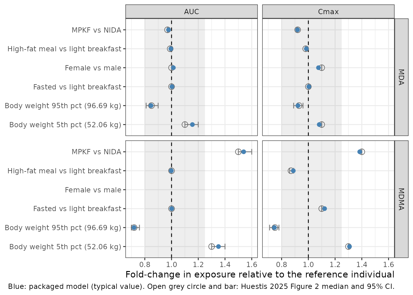
Food-effect study MPKF (Table 1)
A virtual MPKF cohort receives 120 mg MDMA HCl fasted or after a high-fat meal. Body weight is drawn to match Table S4 (mean 78.0 kg, SD 13.4, range 54.7-113.1 kg) with 50% females.
rxode2::rxSetSeed(20251)
set.seed(20251)
n_arm <- 200L

draw_wt <- function(n, mean, sd, lo, hi) {
  meanlog <- log(mean^2 / sqrt(sd^2 + mean^2))
  sdlog <- sqrt(log(1 + sd^2 / mean^2))
  pmin(pmax(rlnorm(n, meanlog, sdlog), lo), hi)
}

obs_grid_mpkf <- c(seq(0, 12, by = 0.25), seq(13, 72, by = 1))

make_cohort <- function(n, id_offset, treatment, amt_mg, wt_mean, wt_sd, wt_lo, wt_hi,
                        pct_female, study_mpkf, fed, fed_highfat, obs_grid) {
  subj <- tibble(
    id = id_offset + seq_len(n),
    treatment = treatment,
    WT = draw_wt(n, wt_mean, wt_sd, wt_lo, wt_hi),
    SEXF = rbinom(n, 1, pct_female / 100),
    STUDY_MPKF = study_mpkf,
    FED = fed,
    FED_HIGHFAT = fed_highfat
  ) |>
    mutate(amt = if (is.function(amt_mg)) amt_mg(WT) else amt_mg)
  bind_rows(
    subj |> mutate(time = 0, evid = 1L, rate = -2, cmt = "depot", dvid = NA_integer_),
    tidyr::expand_grid(subj |> select(-amt), time = obs_grid) |>
      mutate(amt = 0, evid = 0L, rate = 0, cmt = "central", dvid = 1L)
  ) |>
    arrange(id, time, desc(evid))
}

mpkf_events <- bind_rows(
  make_cohort(n_arm, 0L, "Fasted", 120, 78.0, 13.4, 54.7, 113.1, 50, 1, 0, 0, obs_grid_mpkf),
  make_cohort(n_arm, n_arm, "Fed (high-fat)", 120, 78.0, 13.4, 54.7, 113.1, 50, 1, 1, 1, obs_grid_mpkf)
)
stopifnot(!anyDuplicated(unique(mpkf_events[, c("id", "time", "evid")])))

mpkf_sim <- rxode2::rxSolve(mod, events = mpkf_events, keep = "treatment", returnType = "data.frame")
#> ℹ parameter labels from comments will be replaced by 'label()'
mpkf_sim |>
  select(time, treatment, MDMA = Cc, MDA = Cc_tenamfetamine) |>
  pivot_longer(c(MDMA, MDA), names_to = "analyte", values_to = "conc") |>
  group_by(treatment, analyte, time) |>
  summarise(
    p05 = quantile(conc, 0.05), p50 = median(conc), p95 = quantile(conc, 0.95),
    .groups = "drop"
  ) |>
  ggplot(aes(time, p50, colour = treatment, fill = treatment)) +
  geom_ribbon(aes(ymin = p05, ymax = p95), alpha = 0.15, colour = NA) +
  geom_line() +
  facet_wrap(~analyte, scales = "free_y") +
  labs(
    x = "Time after dose (h)", y = "Plasma concentration (ng/mL)",
    colour = NULL, fill = NULL,
    caption = "Median and 90% prediction interval, 120 mg MDMA HCl; virtual MPKF cohort."
  ) +
  theme_bw() +
  theme(legend.position = "bottom")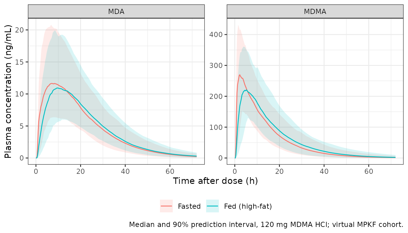
run_nca <- function(sim, conc_col, events) {
  conc <- sim |>
    transmute(id, treatment, time, conc = .data[[conc_col]]) |>
    filter(!is.na(conc))
  conc <- bind_rows(conc, conc |> distinct(id, treatment) |> mutate(time = 0, conc = 0)) |>
    distinct(id, treatment, time, .keep_all = TRUE) |>
    arrange(id, treatment, time)
  dose <- events |>
    filter(evid == 1) |>
    select(id, treatment, time, amt)
  intervals <- data.frame(start = 0, end = Inf, cmax = TRUE, tmax = TRUE, aucinf.obs = TRUE)
  PKNCA::pk.nca(PKNCA::PKNCAdata(
    PKNCA::PKNCAconc(conc, conc ~ time | treatment + id),
    PKNCA::PKNCAdose(dose, amt ~ time | treatment + id),
    intervals = intervals
  ))
}

nca_mdma <- run_nca(mpkf_sim, "Cc", mpkf_events)
nca_mda <- run_nca(mpkf_sim, "Cc_tenamfetamine", mpkf_events)

# Huestis 2025 Table 1, medians (ncaComparisonTable compares medians).
pub_mdma <- tibble::tribble(
  ~treatment,       ~cmax, ~tmax, ~aucinf.obs,
  "Fasted",         234,   2.1,   3729,
  "Fed (high-fat)", 230,   4.0,   3338
)
pub_mda <- tibble::tribble(
  ~treatment,       ~cmax, ~tmax, ~aucinf.obs,
  "Fasted",         12.5,  6.0,   358,
  "Fed (high-fat)", 11.9,  7.0,   343
)
nca_units <- c(cmax = "ng/mL", tmax = "h", aucinf.obs = "ng*h/mL")

cmp_mdma <- nlmixr2lib::ncaComparisonTable(nca_mdma, pub_mdma, by = "treatment", units = nca_units, tolerance_pct = 20)
cmp_mda <- nlmixr2lib::ncaComparisonTable(nca_mda, pub_mda, by = "treatment", units = nca_units, tolerance_pct = 20)
knitr::kable(cmp_mdma, caption = "MDMA, 120 mg MDMA HCl: simulated vs. Huestis 2025 Table 1 medians. * differs by >20%.")| NCA parameter | treatment | Reference | Simulated | % diff |
|---|---|---|---|---|
| Cmax (ng/mL) | Fasted | 234 | 289 | +23.4%* |
| Cmax (ng/mL) | Fed (high-fat) | 230 | 234 | +1.8% |
| Tmax (h) | Fasted | 2.1 | 1.75 | -16.7% |
| Tmax (h) | Fed (high-fat) | 4 | 4.75 | +18.8% |
| AUC0-∞ (obs) (ng*h/mL) | Fasted | 3730 | 4210 | +12.9% |
| AUC0-∞ (obs) (ng*h/mL) | Fed (high-fat) | 3340 | 4230 | +26.6%* |
knitr::kable(cmp_mda, caption = "MDA after 120 mg MDMA HCl: simulated vs. Huestis 2025 Table 1 medians. * differs by >20%.")| NCA parameter | treatment | Reference | Simulated | % diff |
|---|---|---|---|---|
| Cmax (ng/mL) | Fasted | 12.5 | 11.8 | -5.4% |
| Cmax (ng/mL) | Fed (high-fat) | 11.9 | 11.3 | -5.0% |
| Tmax (h) | Fasted | 6 | 8 | +33.3%* |
| Tmax (h) | Fed (high-fat) | 7 | 10.2 | +46.4%* |
| AUC0-∞ (obs) (ng*h/mL) | Fasted | 358 | 326 | -8.9% |
| AUC0-∞ (obs) (ng*h/mL) | Fed (high-fat) | 343 | 317 | -7.7% |
med_sim <- function(nca, code) {
  as.data.frame(nca) |>
    filter(PPTESTCD == code) |>
    group_by(treatment) |>
    summarise(sim = median(PPORRES, na.rm = TRUE), .groups = "drop")
}
gate <- bind_rows(
  med_sim(nca_mdma, "aucinf.obs") |> left_join(rename(pub_mdma, ref = aucinf.obs), by = "treatment") |> mutate(what = "MDMA AUC"),
  med_sim(nca_mdma, "cmax") |> left_join(rename(pub_mdma, ref = cmax), by = "treatment") |> mutate(what = "MDMA Cmax"),
  med_sim(nca_mda, "aucinf.obs") |> left_join(rename(pub_mda, ref = aucinf.obs), by = "treatment") |> mutate(what = "MDA AUC"),
  med_sim(nca_mda, "cmax") |> left_join(rename(pub_mda, ref = cmax), by = "treatment") |> mutate(what = "MDA Cmax")
) |>
  mutate(pct_diff = 100 * (sim / ref - 1))
gate |> select(what, treatment, sim, ref, pct_diff)
#> # A tibble: 8 × 5
#>   what      treatment         sim    ref pct_diff
#>   <chr>     <chr>           <dbl>  <dbl>    <dbl>
#> 1 MDMA AUC  Fasted         4209.  3729      12.9
#> 2 MDMA AUC  Fed (high-fat) 4227.  3338      26.6
#> 3 MDMA Cmax Fasted          289.   234      23.4
#> 4 MDMA Cmax Fed (high-fat)  234.   230       1.84
#> 5 MDA AUC   Fasted          326.   358      -8.87
#> 6 MDA AUC   Fed (high-fat)  317.   343      -7.65
#> 7 MDA Cmax  Fasted           11.8   12.5    -5.39
#> 8 MDA Cmax  Fed (high-fat)   11.3   11.9    -5.05

# Cohort medians against the observed MPKF medians, averaged over the two arms
# for each metric. The model has no food effect on AUC, so the 12% gap between
# the observed fasted and fed AUC medians is sampling noise in 14-15 subjects;
# averaging the arms keeps that noise out of the gate. Dosing the free-base mass
# (84% of the salt) would move every metric by 16%, and a mis-transcribed
# clearance, volume or fm moves it by tens of percent. Realised arm-averaged
# differences: MDMA AUC +20%, MDMA Cmax +13%, MDA AUC -8%, MDA Cmax -5%.
gate_mean <- gate |>
  group_by(what) |>
  summarise(pct_diff = mean(pct_diff), .groups = "drop")
stopifnot(all(abs(gate_mean$pct_diff) < 30))

# Food delays the MDMA peak (Table 1: median Tmax 4.0 h fed vs 2.1 h fasted).
tmax_sim <- med_sim(nca_mdma, "tmax")
stopifnot(tmax_sim$sim[tmax_sim$treatment == "Fed (high-fat)"] -
  tmax_sim$sim[tmax_sim$treatment == "Fasted"] > 1)
The simulated MDMA AUC is 13-27% above the observed MPKF medians (the typical CL/F of an MPKF subject of 76 kg is 28.9 L/h, against 120 mg / 3729 ng*h/mL = 32.2 L/h from the observed fasted median), and the fasted Cmax is the least certain quantity in the model: the fasted effect on ka carries a 72% RSE and a bootstrap median (1.08) well below the point estimate (1.93). MDA AUC and Cmax are reproduced within 10%; the simulated MDA Tmax is 2-3 h later than the observed median, which the sparse MPKF sampling (4, 6, 8 and 12 h) only partly explains.
NIDA study doses (1.0 and 1.6 mg/kg)
The NIDA study arms are summarised in the paper’s reference 8 (Kolbrich 2008, doi:10.1097/FTD.0b013e3181684fa0), whose abstract reports mean MDMA Cmax of 162.9 and 291.8 ng/mL and mean MDA Cmax of 8.4 and 13.8 ng/mL after 1.0 and 1.6 mg/kg MDMA HCl in 17 of the NIDA participants.
obs_grid_nida <- c(seq(0, 12, by = 0.25), seq(13, 167, by = 2))
nida_events <- bind_rows(
  make_cohort(n_arm, 0L, "1.0 mg/kg", function(wt) 1.0 * wt, 72.4, 14.5, 43.1, 99.8, 34.7, 0, 1, 0, obs_grid_nida),
  make_cohort(n_arm, n_arm, "1.6 mg/kg", function(wt) 1.6 * wt, 72.4, 14.5, 43.1, 99.8, 34.7, 0, 1, 0, obs_grid_nida)
)
stopifnot(!anyDuplicated(unique(nida_events[, c("id", "time", "evid")])))
nida_sim <- rxode2::rxSolve(mod, events = nida_events, keep = "treatment", returnType = "data.frame")

nida_cmax <- nida_sim |>
  group_by(treatment, id) |>
  summarise(MDMA = max(Cc), MDA = max(Cc_tenamfetamine), .groups = "drop") |>
  group_by(treatment) |>
  summarise(across(c(MDMA, MDA), mean), .groups = "drop") |>
  mutate(MDMA_ref = c(162.9, 291.8), MDA_ref = c(8.4, 13.8))

nida_cmax |>
  mutate(across(where(is.numeric), ~ signif(.x, 3))) |>
  rename(
    "Dose (MDMA HCl)" = treatment,
    "MDMA Cmax simulated (ng/mL)" = MDMA, "MDMA Cmax Kolbrich 2008 (ng/mL)" = MDMA_ref,
    "MDA Cmax simulated (ng/mL)" = MDA, "MDA Cmax Kolbrich 2008 (ng/mL)" = MDA_ref
  ) |>
knitr::kable(caption = "Mean Cmax in a virtual NIDA cohort versus the Kolbrich 2008 abstract.")| Dose (MDMA HCl) | MDMA Cmax simulated (ng/mL) | MDA Cmax simulated (ng/mL) | MDMA Cmax Kolbrich 2008 (ng/mL) | MDA Cmax Kolbrich 2008 (ng/mL) |
|---|---|---|---|---|
| 1.0 mg/kg | 121 | 8.27 | 163 | 8.4 |
| 1.6 mg/kg | 190 | 13.40 | 292 | 13.8 |
The model under-predicts the NIDA MDMA Cmax, more so at 1.6 mg/kg. Kolbrich 2008 describes MDMA as nonlinear (lower clearance at the higher dose, consistent with MDMA inhibiting its own CYP2D6 metabolism), and the population model has linear clearance, so the dose-dependence is not reproduced. MDA Cmax is close at both doses. These comparisons also bear on the dose basis (see Assumptions and deviations).
Single versus split dosing (Table S5)
The clinical regimen splits the dose, with the second part 1.5-2 h after the first. Huestis 2025 simulated these regimens with the PBPK model only (Table S5: split/single geometric-mean ratio 0.80 for AUC0-4, 1.02-1.03 for AUC0-44, and Cmax 262 vs 277 and 412 vs 431 ng/mL). The same regimens through the population model, for the reference individual:
regimens <- tibble::tribble(
  ~regimen,          ~total, ~amt1, ~amt2,
  "120 mg single",   120,    120,   0,
  "80 + 40 mg",      120,    80,    40,
  "180 mg single",   180,    180,   0,
  "120 + 60 mg",     180,    120,   60
) |>
  mutate(id = row_number(), WT = 70, SEXF = 0, STUDY_MPKF = 0, FED = 1, FED_HIGHFAT = 0)

split_events <- bind_rows(
  regimens |> mutate(time = 0, amt = amt1, evid = 1L, rate = -2, cmt = "depot", dvid = NA_integer_),
  regimens |> filter(amt2 > 0) |> mutate(time = 2, amt = amt2, evid = 1L, rate = -2, cmt = "depot", dvid = NA_integer_),
  tidyr::expand_grid(regimens, time = seq(0, 44, by = 0.01)) |>
    mutate(amt = 0, evid = 0L, rate = 0, cmt = "central", dvid = 1L)
) |>
  select(-amt1, -amt2) |>
  arrange(id, time, desc(evid))

split_sim <- rxode2::rxSolve(mod_typ, split_events, keep = c("regimen", "total"), returnType = "data.frame")
#> ℹ omega/sigma items treated as zero: 'etalcl', 'etalvc', 'etalka', 'etald1', 'etalcl_tenamfetamine', 'etalq_tenamfetamine', 'etalvp_tenamfetamine'
#> Warning: multi-subject simulation without without 'omega'
split_exp <- split_sim |>
  group_by(regimen, total) |>
  summarise(
    AUC0_4 = trap(time[time <= 4], Cc[time <= 4]),
    AUC0_44 = trap(time, Cc),
    Cmax = max(Cc),
    Tmax = time[which.max(Cc)],
    .groups = "drop"
  ) |>
  group_by(total) |>
  mutate(
    ratio_AUC0_4 = AUC0_4 / AUC0_4[grepl("single", regimen)],
    ratio_AUC0_44 = AUC0_44 / AUC0_44[grepl("single", regimen)]
  ) |>
  ungroup() |>
  arrange(match(regimen, regimens$regimen))

split_exp |>
  mutate(across(where(is.numeric), ~ signif(.x, 3))) |>
  select(-total) |>
  rename(
    "Regimen (MDMA HCl)" = regimen, "AUC0-4 (ng*h/mL)" = AUC0_4,
    "AUC0-44 (ng*h/mL)" = AUC0_44, "Cmax (ng/mL)" = Cmax, "Tmax (h)" = Tmax,
    "AUC0-4 split/single" = ratio_AUC0_4, "AUC0-44 split/single" = ratio_AUC0_44
  ) |>
knitr::kable(caption = "Typical-value MDMA exposure for single and split (2 h apart) doses, NIDA reference individual.")| Regimen (MDMA HCl) | AUC0-4 (ng*h/mL) | AUC0-44 (ng*h/mL) | Cmax (ng/mL) | Tmax (h) | AUC0-4 split/single | AUC0-44 split/single |
|---|---|---|---|---|---|---|
| 120 mg single | 614 | 2830 | 210 | 2.86 | 1.000 | 1.000 |
| 80 + 40 mg | 476 | 2820 | 200 | 4.11 | 0.776 | 0.999 |
| 180 mg single | 920 | 4240 | 315 | 2.86 | 1.000 | 1.000 |
| 120 + 60 mg | 714 | 4240 | 300 | 4.11 | 0.776 | 0.999 |
# A split dose delays exposure without changing the total; the PBPK model's
# 0.80 AUC0-4 ratio is the paper's comparison point.
split_ratios <- split_exp |> filter(!grepl("single", regimen))
stopifnot(
  all(abs(split_ratios$ratio_AUC0_44 - 1) < 0.05),
  all(split_ratios$ratio_AUC0_4 > 0.6 & split_ratios$ratio_AUC0_4 < 0.95)
)
The population model reproduces the PBPK result – an AUC0-4 ratio of about 0.8 and an unchanged total – but cannot reproduce the PBPK model’s slightly higher AUC0-44 after a split dose, which arises from time-dependent CYP2D6 inactivation that the linear population model does not contain.
Assumptions and deviations
-
Dose basis. Huestis 2025 states every dose as mg of
MDMA hydrochloride but does not say whether the population PK dataset
recorded the salt or the free-base mass. The packaged model takes the
dose as mg MDMA HCl as administered. With a free-base
dose (193.25 / 229.71 = 0.84 of the salt), the NIDA MDMA Cmax of 162.9
ng/mL at 1.0 mg/kg (Kolbrich 2008) would exceed even an
instantaneous-absorption ceiling of the model (dose / V2/F), and MPKF
and NIDA MDA exposure would be 16-24% below the observed values; with
the salt mass, MDA AUC and Cmax match. The MPKF MDMA AUC alone would
favour the free base, which is recorded here as a known discrepancy. To
simulate a free-base dose, divide it by 0.84 before passing it as
amt. - Absorption structure. The Results describe “a parallel first- and zero-order absorption model”, while the Methods list “first-order and sequential zero-order, followed by first-order absorption” as the candidates and the Discussion describes the final model as “sequential zero- and first-order absorption”. Table 2 lists ka, ALAG1 and D1 but no split fraction, which a parallel model needs. The model is therefore encoded as an absorption lag followed by a zero-order input of duration D1 into the depot and first-order absorption from it (NONMEM ALAG1 and D1 on the depot). The Figure 2 ratios, including the food effects on Cmax, are reproduced with this structure.
-
Prandial covariates. The paper’s three prandial
levels (NIDA light breakfast as reference, MPKF high-fat meal, MPKF
fasted) are encoded with the canonical
FED(1 = any meal) andFED_HIGHFAT(1 = high-fat meal) indicators; the fasted effect is applied as(1 + 1.93 * (1 - FED)). -
Study effect.
STUDY_MPKFcarries the empirical MPKF effect on MDMA CL/F and V2/F and the MPKF additive residual error. The paper regards the effect as an idiosyncrasy of the pooled data; useSTUDY_MPKF = 0for the intended population. -
Metabolite mass units. MDA is formed as
fm * CL/F * C_MDMAwith no molecular-weight conversion, and its concentration is computed from that amount. Becausefmis fixed at 0.1 and the MDA parameters are apparent, any conversion the original analysis applied is absorbed into CLM and V3, and the close match to the observed MDA exposure supports the encoding. - Residual error scale. Table 2 prints the residual-error estimates with concentration units, so they are taken as standard deviations (proportional as a fraction, additive in ng/mL).
- Reference weight. Equation 3 normalises continuous covariates by “median value or a standard value (e.g., 70 kg for body weight)”, and the Figure 2 reference individual weighs 70 kg; 70 kg is used.
-
Covariates screened but not retained (age, albumin,
ALT, creatinine clearance, race; Table S1) are documented in
covariatesDataExcluded. - PBPK model not packaged. The Simcyp model (Table S2) specifies CYP2D6 clearance per pmol of enzyme and time-dependent CYP2D6 inactivation (Ki, kinact), which need the simulator’s enzyme abundance, turnover and organ physiology; those values are not printed, so the PBPK model cannot be reproduced outside Simcyp.
- Virtual cohorts. Body weight is drawn from a log-normal distribution matched to the Table S4 mean and SD and truncated to the observed range; sex follows the Table S4 proportions. The MPKF arms use different virtual subjects rather than a crossover.
- No erratum or correction notice for Huestis 2025 was found in Europe PMC as of 2026-11-02.