Low molecular weight heparin modeling (Schoemaker 1996) • nlmixr2lib

Paper and source

Schoemaker RC, Cohen AF (1996). Estimating impossible curves using NONMEM. Br J Clin Pharmacol 42(3):283–290. doi:10.1046/j.1365-2125.1996.04231.x.

This is a methodology / tutorial paper showing how NONMEM can be applied to data where ordinary nonlinear regression fails. Three worked examples are presented: (1) a rising-dose study of an unnamed anti-hypertensive drug where the lower-dose curves cannot resolve terminal half-life with single-subject regression; (2) intravenous low molecular weight heparin (enoxaparine / Clexane) where anti-Xa activity carries a stubborn basal component that confounds the terminal phase; and (3) intravenous + subcutaneous low molecular weight heparin (dalteparine / Fragmin) where the anti-Xa kinetics and the activated partial thromboplastin time (APTT) pharmacodynamic response are estimated together across both routes.

Example 1’s drug is unnamed and cannot be packaged as a drug-specific nlmixr2lib model; only Examples 2 and 3 are extracted here. The two models live in:

inst/modeldb/specificDrugs/Schoemaker_1996_enoxaparin.R
inst/modeldb/specificDrugs/Schoemaker_1996_dalteparin.R

Anti-Xa observation data for Example 2 come from the upstream cross-over study Stiekema et al. (1993, Br J Clin Pharmacol 35:51–56), and for Example 3 from Kroon et al. (1993, Br J Clin Pharmacol 35:548P). The Schoemaker 1996 fits and parameter estimates are original to that paper; the upstream papers reported only standard NCA-style analyses.

Population

Both Examples were run on the same Centre for Human Drug Research (Leiden) cohort of 12 healthy volunteers, contributing to two independent cross-over studies (one per LMWH series). The Schoemaker 1996 paper does not list baseline demographics directly; both rely on the upstream Stiekema 1993 / Kroon 1993 reports. The population metadata in each model file records what is known and points to the upstream sources.

mod_enox <- readModelDb("Schoemaker_1996_enoxaparin")
mod_dalt <- readModelDb("Schoemaker_1996_dalteparin")
ui_enox  <- rxode2::rxode(mod_enox)
ui_dalt  <- rxode2::rxode(mod_dalt)

c(
  enoxaparin_subjects = ui_enox$population$n_subjects,
  dalteparin_subjects = ui_dalt$population$n_subjects
)
#> enoxaparin_subjects dalteparin_subjects 
#>                  12                  12

Source trace

The per-parameter origin is recorded as an in-file comment next to each ini() entry in both model files. The table below collects them in one place for review.

Enoxaparine (Example 2 / Table 3)

Equation / parameter	Value (paper)	Encoded value	Source location
Equation 9: `C_j = Base + (D/V) * exp(-k * t_j)`	n/a	one-compartment ODE + additive baseline	page 287, Solution 2
`t1/2`	130 min	`lvc = log(6.170 L)` (derived from `CL` and `t1/2`)	Table 3
`CL`	32.9 mL/min	`lcl = log(1.974 L/h)`	Table 3
`Base`	0.0254 IU/mL	`lrbase = log(0.0254)`	Table 3
CV(t1/2)	8.6%	`etalvc` block: 0.02992 (paired with `etalcl`)	Table 3
CV(CL)	15.1%	`etalcl` block: 0.02256	Table 3
CV(Base)	37.7%	`etalrbase ~ 0.1329`	Table 3
s.d. residual error	0.0274 IU/mL	`addSd = 0.0274`	Table 3 footnote

Dalteparine (Example 3 / Table 4)

Equation / parameter	Value (paper)	Encoded value	Source location
Equation 9 (extended with `ka` + depot for SC)	n/a	one-compartment ODE + depot + bioavailability	page 288, Solution-kinetics
Equation 10: `APTT_j = APTT0 * exp((ln(1.1)/I10) * Xa_j)`	n/a	exponential PD on Cc	page 288, Solution-dynamics
`t1/2E`	92.7 min	`lvc = log(6.166 L)` (derived)	Table 4
`t1/2A`	76.6 min	`lka = log(0.5429 1/h)`	Table 4
`CL`	46.1 mL/min	`lcl = log(2.766 L/h)`	Table 4
`F`	70.5%	`lfdepot = log(0.705)`	Table 4
`Base`	0.0192 IU/mL	`lrbase = log(0.0192)`	Table 4
`APTT0`	30.2 s	`lrbase_APTT = log(30.2)`	Table 4
`I10`	0.0665 IU/mL	`lI10 = log(0.0665)`	Table 4
CV(t1/2E)	8.3%	`etalvc` block: 0.02657 (paired with `etalcl`)	Table 4
CV(t1/2A)	0.0%	`ka` typical-value only (no `etalka`)	Table 4
CV(CL)	14.1%	`etalcl` block: 0.01970	Table 4
CV(F)	34.8%	`etalfdepot ~ 0.1143`	Table 4
CV(Base)	16.6%	`etalrbase ~ 0.02719`	Table 4
CV(APTT0)	10.6%	`etalrbase_APTT ~ 0.01117`	Table 4
CV(I10)	19.6%	`etalI10 ~ 0.03770`	Table 4
s.d. residual anti-Xa	0.0207 IU/mL	`addSd = 0.0207`	Table 4 footnote
s.d. residual APTT	1.70 s	`addSd_APTT = 1.70`	Table 4 footnote

Example 2 – Enoxaparine (Clexane)

The paper’s “Solution 2” (the recommended model) is a one-compartment IV bolus model with an estimated constant basal anti-Xa activity:

$C_j = \mathrm{Base} + \frac{D}{V_c} \exp(-k\,t_j)$

The estimated baseline (Base = 0.0254 IU/mL) replaces the pre-value-subtraction and limit-of-quantitation thresholding that the upstream Stiekema 1993 paper applied. The authors argue the basal-activity formulation is to be preferred over the competing two-compartment fit (Solution 1, Table 2) because the implied clearance (32.9 mL/min) matches the dose / AUC clearance Stiekema 1993 reported (26.7 mL/min) far more closely than the two-compartment estimate (9.44 mL/min).

Virtual cohort and simulation

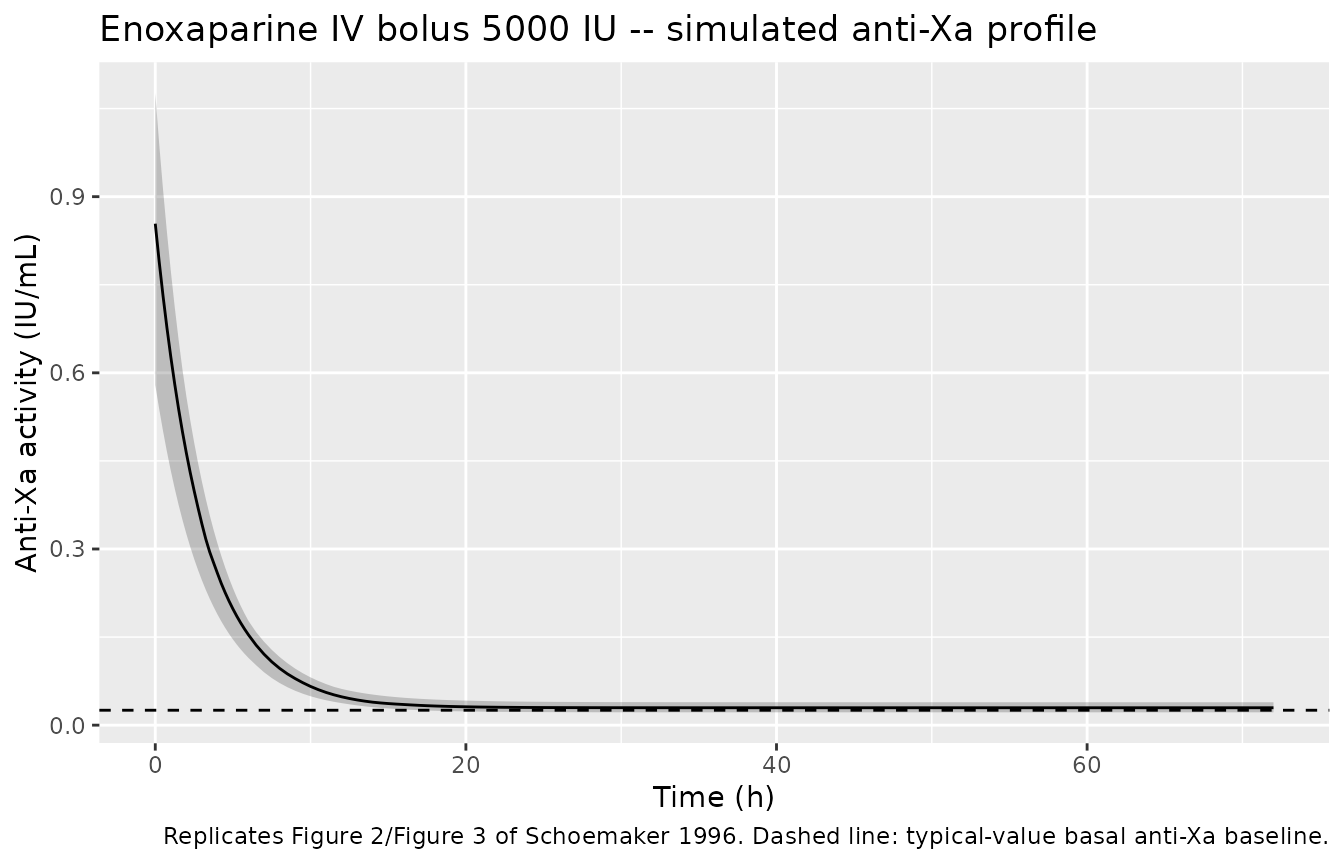
The paper does not list the absolute IV dose used in the upstream Stiekema 1993 study. Figure 2 of Schoemaker 1996 (subject 4) shows peak anti-Xa activity in the 0.4–0.8 IU/mL range, consistent with a single IV bolus of approximately 5000 anti-Xa IU (~50 mg enoxaparin). We use this representative dose below.

set.seed(20260612L)

n_subj <- 12L
dose_iu <- 5000

events_enox <- data.frame(
  id   = seq_len(n_subj),
  time = 0,
  amt  = dose_iu,
  evid = 1L,
  cmt  = "central"
)

# Observation grid (anti-Xa activity), 0 - 72 h covering the Figure 2 window.
obs_times <- c(seq(0, 6, by = 0.25), seq(6.5, 24, by = 0.5), seq(25, 72, by = 1))
obs_enox <- expand.grid(id = seq_len(n_subj), time = obs_times) |>
  dplyr::arrange(id, time) |>
  dplyr::mutate(amt = 0, evid = 0L, cmt = "Cc")

events_enox <- dplyr::bind_rows(events_enox, obs_enox)

sim_enox <- rxode2::rxSolve(
  mod_enox,
  events = events_enox,
  returnType = "data.frame"
)

Replicate Figure 2 / Figure 3

Schoemaker 1996 Figure 3 shows the predicted and observed anti-Xa activity for subjects 4 and 5 over 72 h after Clexane IV. We replicate the predicted profiles (the observed data are not available) by plotting the median and 5th–95th percentile envelope of a typical-dose simulation.

sim_enox |>
  dplyr::group_by(time) |>
  dplyr::summarise(
    Q05 = quantile(Cc, 0.05, na.rm = TRUE),
    Q50 = quantile(Cc, 0.50, na.rm = TRUE),
    Q95 = quantile(Cc, 0.95, na.rm = TRUE),
    .groups = "drop"
  ) |>
  ggplot2::ggplot(ggplot2::aes(time, Q50)) +
  ggplot2::geom_ribbon(ggplot2::aes(ymin = Q05, ymax = Q95), alpha = 0.25) +
  ggplot2::geom_line() +
  ggplot2::geom_hline(yintercept = 0.0254, linetype = "dashed") +
  ggplot2::labs(
    x = "Time (h)", y = "Anti-Xa activity (IU/mL)",
    title = "Enoxaparine IV bolus 5000 IU -- simulated anti-Xa profile",
    caption = "Replicates Figure 2/Figure 3 of Schoemaker 1996. Dashed line: typical-value basal anti-Xa baseline."
  )

PKNCA validation

The Schoemaker 1996 paper does not publish NCA-style summary statistics for Clexane (the comparison was with the upstream Stiekema 1993 dose-by-AUC clearance estimate of 26.7 mL/min). We report the simulated Cmax / Tmax / AUC for the typical-dose IV bolus so a downstream user can sanity-check that the packaged model reproduces sensible exposure metrics. Note: anti-Xa “concentration” here is an activity surrogate (IU/mL), so PKNCA’s clearance computation returns IU per (IU/mL * h) = mL/h dose-units rather than an interpretable mL/h clearance.

sim_nca_enox <- sim_enox |>
  dplyr::filter(!is.na(Cc), time > 0) |>
  dplyr::mutate(treatment = "iv_5000IU") |>
  dplyr::select(id, time, Cc, treatment)

dose_df_enox <- data.frame(
  id        = seq_len(n_subj),
  time      = 0,
  amt       = dose_iu,
  treatment = "iv_5000IU"
)

conc_obj <- PKNCA::PKNCAconc(sim_nca_enox, Cc ~ time | treatment + id,
                             concu = "IU/mL", timeu = "h")
dose_obj <- PKNCA::PKNCAdose(dose_df_enox, amt ~ time | treatment + id,
                             doseu = "IU")

intervals <- data.frame(
  start      = 0,
  end        = Inf,
  cmax       = TRUE,
  tmax       = TRUE,
  aucinf.obs = TRUE,
  half.life  = TRUE
)

nca_enox <- PKNCA::pk.nca(PKNCA::PKNCAdata(conc_obj, dose_obj,
                                           intervals = intervals))
#> Warning: Requesting an AUC range starting (0) before the first measurement (0.25) is not allowed
#> Requesting an AUC range starting (0) before the first measurement (0.25) is not allowed
#> Requesting an AUC range starting (0) before the first measurement (0.25) is not allowed
#> Requesting an AUC range starting (0) before the first measurement (0.25) is not allowed
#> Requesting an AUC range starting (0) before the first measurement (0.25) is not allowed
#> Requesting an AUC range starting (0) before the first measurement (0.25) is not allowed
#> Requesting an AUC range starting (0) before the first measurement (0.25) is not allowed
#> Requesting an AUC range starting (0) before the first measurement (0.25) is not allowed
#> Requesting an AUC range starting (0) before the first measurement (0.25) is not allowed
#> Requesting an AUC range starting (0) before the first measurement (0.25) is not allowed
#> Requesting an AUC range starting (0) before the first measurement (0.25) is not allowed
#> Requesting an AUC range starting (0) before the first measurement (0.25) is not allowed
knitr::kable(as.data.frame(summary(nca_enox)),
             caption = "Schoemaker 1996 enoxaparine: simulated single-dose NCA after 5000 anti-Xa IU IV bolus (12 subjects).")

Schoemaker 1996 enoxaparine: simulated single-dose NCA after 5000 anti-Xa IU IV bolus (12 subjects).
Interval Start	Interval End	treatment	N	Cmax (IU/mL)	Tmax (h)	Half-life (h)	AUCinf,obs (h*IU/mL)
0	Inf	iv_5000IU	12	0.749 [23.0]	0.250 [0.250, 0.250]	1.25e9 [1.41e9]	NC

A typical-individual sanity check (with random effects zeroed out) gives the algebraic peak and half-life directly from ini().

mod_enox_typ <- rxode2::zeroRe(mod_enox)
sim_enox_typ <- rxode2::rxSolve(
  mod_enox_typ,
  events = data.frame(
    id = 1L, time = c(0, 0.001, obs_times[-1]),
    amt = c(dose_iu, rep(0, length(obs_times))),
    evid = c(1L, rep(0L, length(obs_times))),
    cmt  = c("central", rep("Cc", length(obs_times)))
  ),
  returnType = "data.frame"
)
#> ℹ omega/sigma items treated as zero: 'etalcl', 'etalvc', 'etalrbase'

c(
  cmax_typical_IU_per_mL   = round(max(sim_enox_typ$Cc), 4),
  t12_typical_h            = round(log(2) * 6.170 / 1.974, 3),
  rbase_typical_IU_per_mL  = 0.0254
)
#>  cmax_typical_IU_per_mL           t12_typical_h rbase_typical_IU_per_mL 
#>                  0.8355                  2.1670                  0.0254

Example 3 – Dalteparine (Fragmin)

Example 3 extends the basal-activity one-compartment kinetic model with a depot compartment and a bioavailability F for the subcutaneous route, and adds an exponential anti-Xa -> APTT pharmacodynamic sub-model (Equation 10):

$\mathrm{APTT}_j = \mathrm{APTT_0}\,\exp\!\left(\frac{\ln 1.1}{I_{10}}\,\mathrm{Xa}_j\right) + \varepsilon_{2j}$

The I10 parameter is the anti-Xa activity increment required to produce a 10% rise in APTT relative to its baseline APTT0. The parameter estimates in Table 4 come from a final joint IV+SC fit with all parameters free (the unrestricted analysis in the paper’s Solution-kinetics paragraph).

Virtual cohort and simulation (IV + SC)

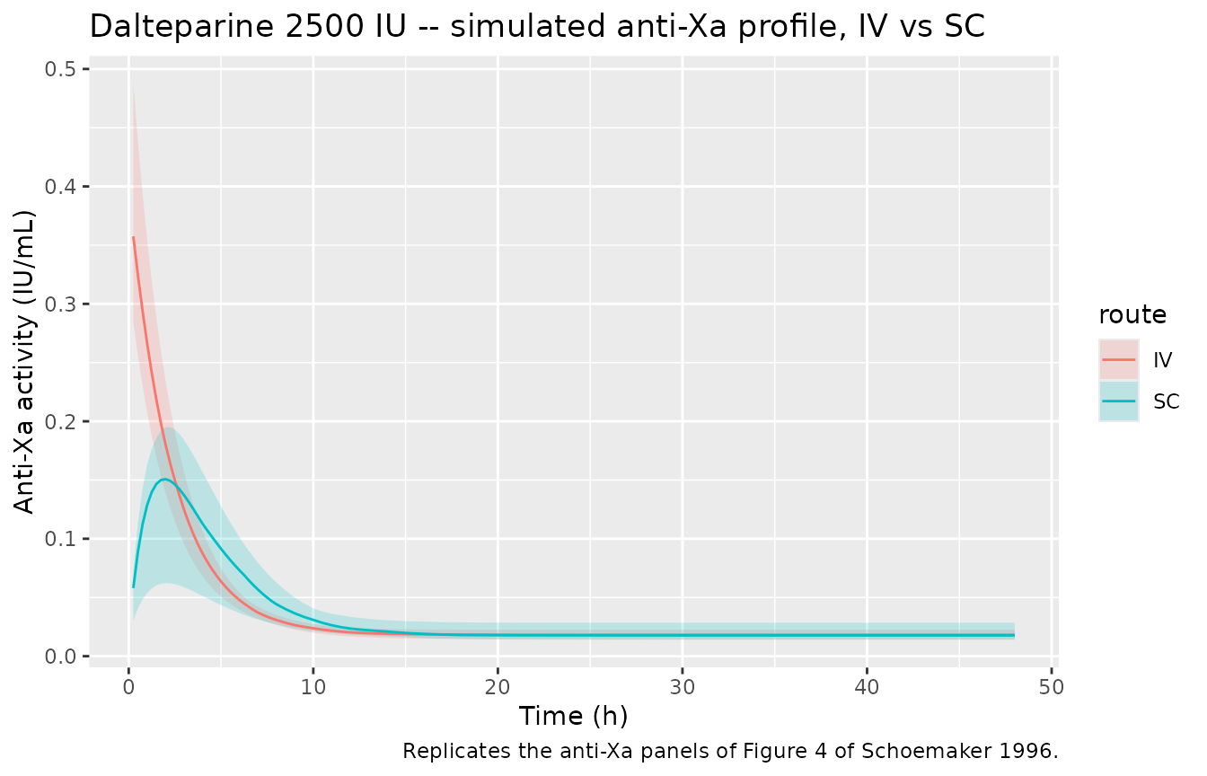
Figure 4 of Schoemaker 1996 plots subject 3’s IV and SC profiles. Peak anti-Xa activity in Figure 4 is ~0.3–0.4 IU/mL, consistent with an IV dose of approximately 2500 anti-Xa IU. We simulate both routes at this representative dose so the predicted Cc and APTT trajectories match the figure’s scale.

set.seed(20260612L)

n_subj_d <- 12L
dose_iu_d <- 2500

# IV cohort
events_iv <- data.frame(
  id   = seq_len(n_subj_d),
  time = 0,
  amt  = dose_iu_d,
  evid = 1L,
  cmt  = "central"
)
# SC cohort -- IDs offset to avoid id collisions
events_sc <- data.frame(
  id   = n_subj_d + seq_len(n_subj_d),
  time = 0,
  amt  = dose_iu_d,
  evid = 1L,
  cmt  = "depot"
)

obs_times_d <- c(seq(0, 8, by = 0.25), seq(8.5, 24, by = 0.5),
                 seq(25, 48, by = 1))

# Observations for both Cc and APTT
make_obs <- function(ids, route_label) {
  expand.grid(id = ids, time = obs_times_d, cmt = c("Cc", "APTT"),
              stringsAsFactors = FALSE) |>
    dplyr::arrange(id, time) |>
    dplyr::mutate(amt = 0, evid = 0L, route = route_label)
}

obs_iv <- make_obs(seq_len(n_subj_d), "IV")
obs_sc <- make_obs(n_subj_d + seq_len(n_subj_d), "SC")

events_iv$route <- "IV"
events_sc$route <- "SC"

events_dalt <- dplyr::bind_rows(events_iv, events_sc, obs_iv, obs_sc)
stopifnot(!anyDuplicated(unique(events_dalt[, c("id", "time", "evid", "cmt")])))

sim_dalt <- rxode2::rxSolve(
  mod_dalt,
  events = events_dalt,
  keep   = c("route"),
  returnType = "data.frame"
)

Replicate Figure 4 – anti-Xa profiles by route

sim_dalt |>
  dplyr::filter(!is.na(Cc), time > 0) |>
  dplyr::group_by(time, route) |>
  dplyr::summarise(
    Q05 = quantile(Cc, 0.05, na.rm = TRUE),
    Q50 = quantile(Cc, 0.50, na.rm = TRUE),
    Q95 = quantile(Cc, 0.95, na.rm = TRUE),
    .groups = "drop"
  ) |>
  ggplot2::ggplot(ggplot2::aes(time, Q50, colour = route, fill = route)) +
  ggplot2::geom_ribbon(ggplot2::aes(ymin = Q05, ymax = Q95),
                       alpha = 0.2, colour = NA) +
  ggplot2::geom_line() +
  ggplot2::labs(
    x = "Time (h)", y = "Anti-Xa activity (IU/mL)",
    title = "Dalteparine 2500 IU -- simulated anti-Xa profile, IV vs SC",
    caption = "Replicates the anti-Xa panels of Figure 4 of Schoemaker 1996."
  )

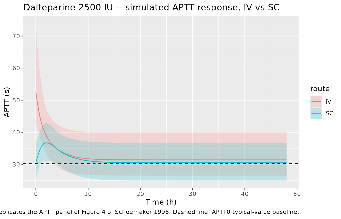
Replicate Figure 4 – APTT response by route

sim_dalt |>
  dplyr::filter(!is.na(APTT), time >= 0) |>
  dplyr::group_by(time, route) |>
  dplyr::summarise(
    Q05 = quantile(APTT, 0.05, na.rm = TRUE),
    Q50 = quantile(APTT, 0.50, na.rm = TRUE),
    Q95 = quantile(APTT, 0.95, na.rm = TRUE),
    .groups = "drop"
  ) |>
  ggplot2::ggplot(ggplot2::aes(time, Q50, colour = route, fill = route)) +
  ggplot2::geom_ribbon(ggplot2::aes(ymin = Q05, ymax = Q95),
                       alpha = 0.2, colour = NA) +
  ggplot2::geom_line() +
  ggplot2::geom_hline(yintercept = 30.2, linetype = "dashed") +
  ggplot2::labs(
    x = "Time (h)", y = "APTT (s)",
    title = "Dalteparine 2500 IU -- simulated APTT response, IV vs SC",
    caption = "Replicates the APTT panel of Figure 4 of Schoemaker 1996. Dashed line: APTT0 typical-value baseline."
  )

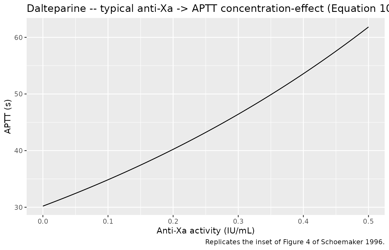
Replicate Figure 4 – anti-Xa to APTT concentration-effect curve

The inset of Figure 4 plots APTT against the (predicted) anti-Xa activity for the same subject. We reproduce the typical-value concentration-effect curve directly from Equation 10.

xa_grid <- seq(0, 0.5, length.out = 201)
aptt_typ <- 30.2 * exp((log(1.1) / 0.0665) * xa_grid)

data.frame(Cc = xa_grid, APTT = aptt_typ) |>
  ggplot2::ggplot(ggplot2::aes(Cc, APTT)) +
  ggplot2::geom_line() +
  ggplot2::labs(
    x = "Anti-Xa activity (IU/mL)",
    y = "APTT (s)",
    title = "Dalteparine -- typical anti-Xa -> APTT concentration-effect (Equation 10)",
    caption = "Replicates the inset of Figure 4 of Schoemaker 1996."
  )

PKNCA validation – anti-Xa

The paper does not publish NCA statistics for the dalteparine arm either; the table below is the simulated single-dose summary for both routes. The IV/SC pair is what tests the structural fit (bioavailability and absorption-time combine multiplicatively into the AUC ratio, which should equal F = 0.705).

sim_nca_dalt <- sim_dalt |>
  dplyr::filter(!is.na(Cc), time > 0) |>
  dplyr::select(id, time, Cc, route) |>
  dplyr::distinct(id, time, route, .keep_all = TRUE) |>
  dplyr::rename(treatment = route)

dose_df_dalt <- data.frame(
  id        = c(events_iv$id, events_sc$id),
  time      = 0,
  amt       = dose_iu_d,
  treatment = c(events_iv$route, events_sc$route)
)

conc_obj_d <- PKNCA::PKNCAconc(sim_nca_dalt, Cc ~ time | treatment + id,
                               concu = "IU/mL", timeu = "h")
dose_obj_d <- PKNCA::PKNCAdose(dose_df_dalt, amt ~ time | treatment + id,
                               doseu = "IU")

intervals_d <- data.frame(
  start      = 0,
  end        = Inf,
  cmax       = TRUE,
  tmax       = TRUE,
  aucinf.obs = TRUE,
  half.life  = TRUE
)

nca_dalt <- PKNCA::pk.nca(PKNCA::PKNCAdata(conc_obj_d, dose_obj_d,
                                           intervals = intervals_d))
#> Warning: Requesting an AUC range starting (0) before the first measurement (0.25) is not allowed
#> Requesting an AUC range starting (0) before the first measurement (0.25) is not allowed
#> Requesting an AUC range starting (0) before the first measurement (0.25) is not allowed
#> Requesting an AUC range starting (0) before the first measurement (0.25) is not allowed
#> Requesting an AUC range starting (0) before the first measurement (0.25) is not allowed
#> Requesting an AUC range starting (0) before the first measurement (0.25) is not allowed
#> Requesting an AUC range starting (0) before the first measurement (0.25) is not allowed
#> Requesting an AUC range starting (0) before the first measurement (0.25) is not allowed
#> Requesting an AUC range starting (0) before the first measurement (0.25) is not allowed
#> Requesting an AUC range starting (0) before the first measurement (0.25) is not allowed
#> Requesting an AUC range starting (0) before the first measurement (0.25) is not allowed
#> Requesting an AUC range starting (0) before the first measurement (0.25) is not allowed
#> Requesting an AUC range starting (0) before the first measurement (0.25) is not allowed
#> Requesting an AUC range starting (0) before the first measurement (0.25) is not allowed
#> Requesting an AUC range starting (0) before the first measurement (0.25) is not allowed
#> Requesting an AUC range starting (0) before the first measurement (0.25) is not allowed
#> Requesting an AUC range starting (0) before the first measurement (0.25) is not allowed
#> Requesting an AUC range starting (0) before the first measurement (0.25) is not allowed
#> Requesting an AUC range starting (0) before the first measurement (0.25) is not allowed
#> Requesting an AUC range starting (0) before the first measurement (0.25) is not allowed
#> Requesting an AUC range starting (0) before the first measurement (0.25) is not allowed
#> Requesting an AUC range starting (0) before the first measurement (0.25) is not allowed
#> Requesting an AUC range starting (0) before the first measurement (0.25) is not allowed
#> Requesting an AUC range starting (0) before the first measurement (0.25) is not allowed
knitr::kable(as.data.frame(summary(nca_dalt)),
             caption = "Schoemaker 1996 dalteparine: simulated single-dose NCA after 2500 anti-Xa IU IV vs SC (12 subjects per route).")

Schoemaker 1996 dalteparine: simulated single-dose NCA after 2500 anti-Xa IU IV vs SC (12 subjects per route).
Interval Start	Interval End	treatment	N	Cmax (IU/mL)	Tmax (h)	Half-life (h)	AUCinf,obs (h*IU/mL)
0	Inf	IV	12	0.361 [15.2]	0.250 [0.250, 0.250]	8.39e7 [1.02e8]	NC
0	Inf	SC	12	0.134 [36.5]	2.00 [1.75, 2.25]	5.82e7 [8.58e7]	NC

Assumptions and deviations

Dose amounts: Schoemaker 1996 does not list the absolute IV / SC doses used in the upstream Stiekema 1993 / Kroon 1993 studies. The vignette uses 5000 anti-Xa IU IV for enoxaparine and 2500 anti-Xa IU for dalteparine (both routes), values chosen by visual back-fit against the peak anti-Xa activity in Figures 2–4 of Schoemaker 1996. This is a simulation choice to make the figures match – it is not a fit to the published dose specification, which would require the upstream papers on disk.
IIV reparameterisation: Schoemaker 1996 parameterises in (CL, t1/2) (Example 2) and (CL, t1/2E, t1/2A, F, Base, APTT0, I10) (Example 3), with independent etas on each. The packaged models use the nlmixr2lib-canonical (CL, Vc) parameterisation, with the implied joint distribution Var(eta_lvc) = Var(eta_lcl) + Var(eta_lt12) and Cov(eta_lcl, eta_lvc) = Var(eta_lcl) encoded as a 2x2 block matrix. This reproduces the paper’s reported CV on CL, t1/2, and t1/2E exactly when the block is sampled; it changes the marginal CV on Vc (which the paper does not report).
No covariates: the Schoemaker 1996 paper does not test or report any covariate effects on the LMWH PK parameters. covariateData is empty in both model files; downstream users wishing to add allometric scaling on weight would need to extend the model file.
No NCA comparison table: Schoemaker 1996 does not publish Cmax / Tmax / AUC / half-life NCA values for either Clexane or Fragmin. The closest reference value is the Stiekema 1993 dose-by-AUC clearance estimate of 26.7 mL/min for Clexane (vs the packaged enoxaparine model’s typical CL of 32.9 mL/min); the difference is attributed by the Schoemaker authors to the area Solution 1 attributes to the (absent in Solution 2) second compartment.
APTT as PD output: Schoemaker 1996 implemented Equation 10 with the empirical-Bayes anti-Xa estimates supplied to NONMEM as covariates driving APTT, not as a joint two-output likelihood. The packaged nlmixr2lib model uses the model-predicted Cc (state-derived) as the input to the exponential APTT predictor, which is the natural nlmixr2 / rxode2 two-output formulation. For typical-value forward simulation the two encodings agree; for VPC or re-fitting the small difference between empirical-Bayes Xa and model-predicted Xa as the PD driver is not reproduced.
Example 1 not packaged: the rising-dose anti-hypertensive example (Table 1) uses an unnamed drug and therefore cannot be packaged as a drug-specific model under inst/modeldb/specificDrugs/. Its parameters (t1/2_alpha = 4.80 min, t1/2_beta = 362 min, Vc = 32.7 L, CL = 155 mL/min, CV_residual = 23.1%) are recorded here for completeness only; they are not loadable through readModelDb().