Tecovirimat (ST-246) animal-rule dose selection (Leeds 2013)
Source:vignettes/articles/Leeds_2013_tecovirimat.Rmd
Leeds_2013_tecovirimat.RmdModel and source
Leeds 2013 is an “animal rule” (21 CFR 314.600) dose-selection paper for tecovirimat, then known by its development code ST-246, a smallpox therapeutic. Because smallpox is eradicated there is no human efficacy population, so the efficacious human dose was chosen by bridging efficacy in monkeypox-virus (MPXV) infected cynomolgus monkeys to human exposure through a pair of population PK models. The paper therefore contributes two independent fits, extracted here as two model files.
cyno_ui  <- rxode2::rxode(readModelDb("Leeds_2013_tecovirimat_cyno"))
#> ℹ parameter labels from comments will be replaced by 'label()'
#> Warning: some etas defaulted to non-mu referenced, possible parsing error: etaiov_ka_1, etaiov_ka_2, etaiov_cl_1, etaiov_cl_2
#> as a work-around try putting the mu-referenced expression on a simple line
human_ui <- rxode2::rxode(readModelDb("Leeds_2013_tecovirimat_human"))
#> ℹ parameter labels from comments will be replaced by 'label()'- Citation: Leeds JM, Fenneteau F, Gosselin NH, Mouksassi MS, Kassir N, Marier JF, Chen Y, Grosenbach D, Frimm AE, Honeychurch KM, Chinsangaram J, Tyavanagimatt SR, Hruby DE, Jordan R. (2013). Pharmacokinetic and pharmacodynamic modeling to determine the dose of ST-246 to protect against smallpox in humans. Antimicrob Agents Chemother 57(3):1136-1143. doi:10.1128/AAC.00959-12.
- Cynomolgus-monkey model: Preclinical (cynomolgus monkey). Two-compartment population PK model for oral tecovirimat (ST-246) in uninfected and monkeypox-virus-infected cynomolgus monkeys (Leeds 2013), with first-order absorption preceded by a lag time, allometric body-weight scaling (0.75 on CL/F and Q/F, 1 on Vc/F and Vp/F) about a 3.105 kg median weight, a weight-adjusted dose-level power effect on Ka, CL/F and Vc/F, an infection-status effect on Ka and CL/F, and two-occasion inter-occasion variability on Ka and CL/F. Companion human model: modellib(‘Leeds_2013_tecovirimat_human’).
- Human model: Two-compartment population PK model for oral tecovirimat (ST-246) in healthy adult volunteers (Leeds 2013), with first-order absorption preceded by a lag time, allometric body-weight scaling (0.75 on CL/F and Q/F, 1 on Vc/F and Vp/F) about a 78.4 kg mean weight, and a sex effect on Vc/F (29.5% larger apparent central volume in women). Companion cynomolgus-monkey model used for the animal-rule dose bridge: modellib(‘Leeds_2013_tecovirimat_cyno’).
- Article: https://doi.org/10.1128/AAC.00959-12
Both fits are two-compartment models with first-order oral absorption preceded by a lag time, fit in Phoenix NLME 6.2.0.416 with FOCE-ELS, and both scale allometrically on body weight with theory-based exponents (0.75 on the clearance terms, 1 on the volume terms). They differ in exactly the two ways the paper states: the human model carries a sex effect on the apparent central volume, and the monkey model carries a weight-adjusted dose-level effect on Ka, CL/F and Vc/F plus an infection-status effect on Ka and CL/F.
The paper’s pharmacodynamic analysis (Kaplan-Meier survival, Cox proportional-hazards testing and recursive ROC analysis across 96 monkeys) is nonparametric – it fits no hazard function and publishes no PD parameters – so it contributes no third model file. Its outputs are exposure cutoffs, and those are used below as validation targets for the PK models.
Population
Cynomolgus monkeys. Six studies. Study 1 was a GLP PK study in uninfected animals dosed once daily at 0.3, 3, 10, 20 and 30 mg/kg (n = 6 per dose, 3 male and 3 female). Study 2 determined the effect of infection, dosing 3, 10 or 20 mg/kg (n = 6 per group) from day 4 after inoculation, with a single dose given 10 days before inoculation so that infected and uninfected PK could be compared within animal. Studies 3-6 were efficacy studies with sparse PK, dosing 0.3 to 300 mg/kg for 14 consecutive days starting 3, 4 or 5 days after infection. Infection was intravenous inoculation with approximately 5e7 PFU of MPXV per animal, which is nearly uniformly lethal with a median time to death of 14 days. The model’s weight normalisation constant, 3.105 kg, is the cohort median. 1,558 plasma concentrations entered the population PK analysis (21 of 1,579 non-BQL concentrations excluded as outliers), none with an absolute CWRES above 4.
Humans. One double-blind, randomised, placebo-controlled, multicentre phase 1 trial. 107 healthy volunteers aged 19 to 74 with approximately equal numbers of men and women were randomised to 400 mg (45 subjects), 600 mg (46 subjects) or placebo (16 subjects) once daily for 14 days in the nonfasted state, so 91 subjects contribute concentrations. Subjects with fewer than two concentrations were excluded (3 in total), as were outliers with high troughs or double peaks at 24 h. 1,395 concentrations entered the analysis, none with an absolute CWRES above 4. Below-quantitation-limit values were handled by Beal’s method M6. The model’s weight normalisation constant, 78.4 kg, is the cohort mean weight.
The same information is available programmatically from each model’s
population metadata.
str(human_ui$population, max.level = 1)
#> List of 9
#>  $ species       : chr "human"
#>  $ n_subjects    : int 91
#>  $ n_studies     : int 1
#>  $ age_range     : chr "19-74 years"
#>  $ weight_mean   : chr "78.4 kg"
#>  $ sex_female_pct: num 50
#>  $ disease_state : chr "Healthy volunteers."
#>  $ dose_range    : chr "Oral ST-246 400 mg (45 subjects) or 600 mg (46 subjects) once daily for 14 days, administered in the nonfasted state."
#>  $ notes         : chr "Double-blind, randomised, placebo-controlled, multicenter phase 1 safety / tolerability / PK trial; 107 volunte"| __truncated__
Source trace
Every ini() entry in both model files carries an in-file
comment naming its source location. They are collected here for review.
All values come from Table 1 of Leeds 2013, “Population
pharmacokinetic parameters for the 2-compartment model that best fit the
pharmacokinetic data for both cynomolgus monkeys (NHPs) and humans…”,
verified against the published PDF rather than against an extracted-text
rendering of it.
Cynomolgus-monkey model
| Parameter | Value as encoded | Source location |
|---|---|---|
lka |
log(0.586) |
Table 1 row Ka (h-1), NHP Uninfected:
0.586 * (dose/10)^0.160
|
e_dis_infect_active_ka |
log(0.868 / 0.586) |
Table 1 row Ka (h-1), NHP Infected 0.868 vs Uninfected
0.586 |
e_dose_tecovirimat_mgkg_ka |
0.160 |
Table 1 row Ka (h-1), NHP, both statuses |
ltlag |
log(0.302) |
Table 1 row Tlag (h), NHP = 0.302 |
lcl |
log(2.827) |
Table 1 row CL/F (liters/h), NHP Uninfected:
2.827 * (wt/3.105)^0.75 * (dose/10)^0.093
|
e_dis_infect_active_cl |
log(2.809 / 2.827) |
Table 1 row CL/F (liters/h), NHP Infected 2.809 vs
Uninfected 2.827 |
e_dose_tecovirimat_mgkg_cl |
0.093 |
Table 1 row CL/F (liters/h), NHP, both statuses |
lvc |
log(20.054) |
Table 1 row Vc/F (liters), NHP:
20.054 * (wt/3.105)^1 * (dose/10)^0.623
|
e_dose_tecovirimat_mgkg_vc |
0.623 |
Table 1 row Vc/F (liters), NHP |
lq |
log(3.244) |
Table 1 row Q/F (liters/h), NHP:
3.244 * (wt/3.105)^0.75
|
lvp |
log(13.34) |
Table 1 row Vp/F (liters), NHP:
13.34 * (wt/3.105)
|
e_wt_cl_q |
fixed(0.75) |
Results, “NHP POP PK model development”: theta_eff 0.75 for clearance-related parameters |
e_wt_vc_vp |
fixed(1.0) |
Results, “NHP POP PK model development”: theta_eff 1 for volume-related parameters |
etalka, etalcl, etalvc,
etalq, etalvp
|
0.11^2, 0.31^2, 0.47^2,
0.75^2, 0.55^2
|
Table 1 column IIV (%), NHP: 11, 31, 47, 75, 55 |
etaiov_ka_1/2, etaiov_cl_1/2
|
0.32^2, 0.14^2
|
Table 1 column IOV (%), NHP: 32 on Ka, 14 on CL/F |
propSd |
0.30 |
Table 1 Error model / Proportional (%), NHP = 30 |
addSd |
0.133 / 1000 |
Table 1 Error model / Additive (ug/liter), NHP = 0.133,
converted to mg/L |
| ODE structure | n/a | Results, “NHP POP PK model development”: “2-compartment model with correlation between CL/F and Vc/F and a lag time in absorption (Tlag)” |
Human model
| Parameter | Value as encoded | Source location |
|---|---|---|
lka |
log(1.06) |
Table 1 row Ka (h-1), Human = 1.06 |
ltlag |
log(1.46) |
Table 1 row Tlag (h), Human = 1.46 |
lcl |
log(41.15) |
Table 1 row CL/F (liters/h), Human:
41.15 * (wt/78.4)^0.75
|
lvc |
log(217.44) |
Table 1 row Vc/F (liters), Human:
217.44 * (wt/78.4)^1 (male)
|
e_sexf_vc |
log(281.51 / 217.44) |
Table 1 row Vc/F (liters), Human: 281.51 (female) vs
217.44 (male) |
lq |
log(36.79) |
Table 1 row Q/F (liters/h), Human:
36.79 * (wt/78.4)^0.75
|
lvp |
log(413.53) |
Table 1 row Vp/F (liters), Human:
413.53 * (wt/78.4)^1
|
e_wt_cl_q |
fixed(0.75) |
Table 1 human CL/F and Q/F formulae; Results, “Human POP PK model development”: allometric factors “similar to the NHP model” |
e_wt_vc_vp |
fixed(1.0) |
Table 1 human Vc/F and Vp/F formulae |
etalka, etaltlag, etalcl,
etalvc, etalq, etalvp
|
0.41^2, 0.17^2, 0.31^2,
0.28^2, 0.54^2, 0.54^2
|
Table 1 column IIV (%), Human: 41, 17, 31, 28, 54,
54 |
propSd |
0.27 |
Table 1 Error model / Proportional (%), Human = 27 |
addSd |
10.92 / 1000 |
Table 1 Error model / Additive (ug/liter), Human =
10.92, converted to mg/L |
Structural check: typical-value terminal half-life
The strongest transcription check the paper offers costs no simulation assumptions at all. Results, “Human POP PK model development” states: “The terminal elimination half-lives in male and female subjects were similar (16.7 h in males versus 17.4 h in females).” For a two-compartment model that number is a joint function of CL/F, Vc/F, Q/F and Vp/F, and the male-female difference is driven only by the sex effect on Vc/F – so reproducing both values simultaneously exercises five of the seven human structural parameters.
beta_thalf <- function(cl, vc, q, vp) {
  k10 <- cl / vc; k12 <- q / vc; k21 <- q / vp
  a <- k10 + k12 + k21
  beta <- (a - sqrt(a^2 - 4 * k10 * k21)) / 2
  log(2) / beta
}
th_male   <- beta_thalf(41.15, 217.44, 36.79, 413.53)
th_female <- beta_thalf(41.15, 281.51, 36.79, 413.53)

# Deterministic quantities computed from the published typical values -- no
# cohort is involved, so a tight bound is the correct assertion here.
stopifnot(
  abs(th_male   - 16.7) < 0.1,
  abs(th_female - 17.4) < 0.1
)
data.frame(
  Sex        = c("Male", "Female"),
  Published  = c(16.7, 17.4),
  Reproduced = round(c(th_male, th_female), 2)
) |>
knitr::kable(caption = "Terminal elimination half-life (h), Leeds 2013 Results vs the packaged model.")| Sex | Published | Reproduced |
|---|---|---|
| Male | 16.7 | 16.71 |
| Female | 17.4 | 17.37 |
Virtual cohorts
Original observed data are not publicly available. The simulations below use virtual populations whose covariate distributions approximate the published demographics. Leeds 2013 reports only the central body weight for each species (78.4 kg mean in humans, 3.105 kg median in monkeys) and no dispersion, so the spread is assumed; see “Assumptions and deviations”.
# `set.seed()` seeds R's RNG only. rxode2 partitions its own simulation streams
# per solver thread, so this cohort is NOT reproducible across machines with
# different thread counts. Every assertion on a cohort-derived quantity below
# is written to hold for any cohort the model can produce.
set.seed(20130301)
rxode2::rxSetSeed(20130301)

N_HUMAN <- 200L  # per arm; the cohort cap
N_CYNO  <- 100L  # per arm; 5 monkey arms are needed for the dose bridge

TAU  <- 24                            # once-daily
DOSE_TIMES <- seq(0, 13 * TAU, by = TAU)   # 14 daily doses
SS_START   <- max(DOSE_TIMES)              # 312 h, the final dose
# Day-1 and final-interval observation windows, on a grid fine enough that the
# trapezoidal AUC does not lose the peak.
OBS_TIMES <- c(seq(0, TAU, by = 0.25), seq(SS_START, SS_START + TAU, by = 0.25))

make_cohort <- function(n, amt_fun, covariates, treatment, id_offset = 0L) {
  subj <- tibble::tibble(id = id_offset + seq_len(n), treatment = treatment)
  for (nm in names(covariates)) subj[[nm]] <- covariates[[nm]](n)
  subj$amt_per_dose <- amt_fun(subj)
  doses <- subj |>
    tidyr::crossing(time = DOSE_TIMES) |>
    dplyr::mutate(evid = 1L, cmt = "depot", amt = amt_per_dose)
  obs <- subj |>
    tidyr::crossing(time = OBS_TIMES) |>
    dplyr::mutate(evid = 0L, cmt = "central", amt = NA_real_)
  dplyr::bind_rows(doses, obs) |>
    dplyr::select(-amt_per_dose) |>
    dplyr::arrange(id, time, dplyr::desc(evid))
}

# Human body weight: lognormal with the published 78.4 kg centre and an assumed
# 18% CV; sex assigned 50/50 to match "approximately equal numbers".
human_cov <- list(
  WT   = function(n) 78.4 * exp(stats::rnorm(n, 0, 0.18)),
  SEXF = function(n) rep(c(0, 1), length.out = n)
)
human_events <- dplyr::bind_rows(
  make_cohort(N_HUMAN, function(d) 400, human_cov, "Human 400 mg", id_offset =   0L),
  make_cohort(N_HUMAN, function(d) 600, human_cov, "Human 600 mg", id_offset = 200L)
)

# Monkey arms spanning the paper's two published exposure-equivalence bands
# (8-10 mg/kg for 400 mg, 12-14 mg/kg for 600 mg) plus the lowest efficacious
# dose (3 mg/kg). Uninfected, matching the direct comparison of Figure 4A.
CYNO_LEVELS <- c(3, 8, 10, 12, 14)
cyno_events <- dplyr::bind_rows(lapply(seq_along(CYNO_LEVELS), function(i) {
  lvl <- CYNO_LEVELS[i]
  make_cohort(
    N_CYNO,
    amt_fun = function(d) lvl * d$WT,
    covariates = list(
      WT                    = function(n) 3.105 * exp(stats::rnorm(n, 0, 0.12)),
      DIS_INFECT_ACTIVE     = function(n) rep(0, n),
      OCC                   = function(n) rep(1, n),
      DOSE_TECOVIRIMAT_MGKG = function(n) rep(lvl, n)
    ),
    treatment = sprintf("NHP %g mg/kg", lvl),
    id_offset = 1000L + (i - 1L) * N_CYNO
  )
}))

stopifnot(
  !anyDuplicated(unique(human_events[, c("id", "time", "evid")])),
  !anyDuplicated(unique(cyno_events[, c("id", "time", "evid")]))
)
Simulation
human_sim <- rxode2::rxSolve(
  human_ui, human_events,
  keep = c("treatment", "WT", "SEXF")
) |> as.data.frame()

cyno_sim <- rxode2::rxSolve(
  cyno_ui, cyno_events,
  keep = c("treatment", "WT", "DOSE_TECOVIRIMAT_MGKG")
) |> as.data.frame()

# Solver-noise guard: a concentration that has decayed below zero would make
# PKNCA's log-linear steps return NaN.
stopifnot(
  all(human_sim$Cc[!is.na(human_sim$Cc)] >= 0),
  all(cyno_sim$Cc[!is.na(cyno_sim$Cc)]   >= 0)
)
Replicate Figure 4A: steady-state concentration-time curves
Figure 4A of Leeds 2013 overlays steady-state plasma concentration-time curves for 400 mg and 600 mg in healthy humans against 3 mg/kg and 10 mg/kg in uninfected monkeys, and the paper reads it as: “the 400-mg human plasma concentration-time curve was essentially identical to the 10-mg/kg NHP curve, while that for the 600-mg dose was slightly higher. Concentrations at all time points for both human doses were substantially higher than those of the lowest efficacious dose for NHPs, 3 mg/kg.”
fig4a <- dplyr::bind_rows(
  human_sim |> dplyr::filter(treatment %in% c("Human 400 mg", "Human 600 mg")),
  cyno_sim  |> dplyr::filter(treatment %in% c("NHP 3 mg/kg", "NHP 10 mg/kg"))
) |>
  dplyr::filter(time >= SS_START, !is.na(Cc)) |>
  dplyr::mutate(
    tad     = time - SS_START,
    species = ifelse(grepl("^Human", treatment), "Human", "Cynomolgus monkey")
  ) |>
  dplyr::group_by(species, treatment, tad) |>
  dplyr::summarise(Cc = mean(Cc), .groups = "drop")

ggplot(fig4a, aes(tad, Cc, colour = treatment, linetype = species)) +
  geom_line(linewidth = 0.7) +
  scale_y_log10() +
  labs(
    x = "Time after the day-14 dose (h)", y = "Tecovirimat (mg/L)",
    colour = NULL, linetype = NULL,
    title = "Steady-state concentration-time curves",
    caption = "Replicates Figure 4A of Leeds 2013 (mean profiles, uninfected)."
  ) +
  theme(legend.position = "bottom")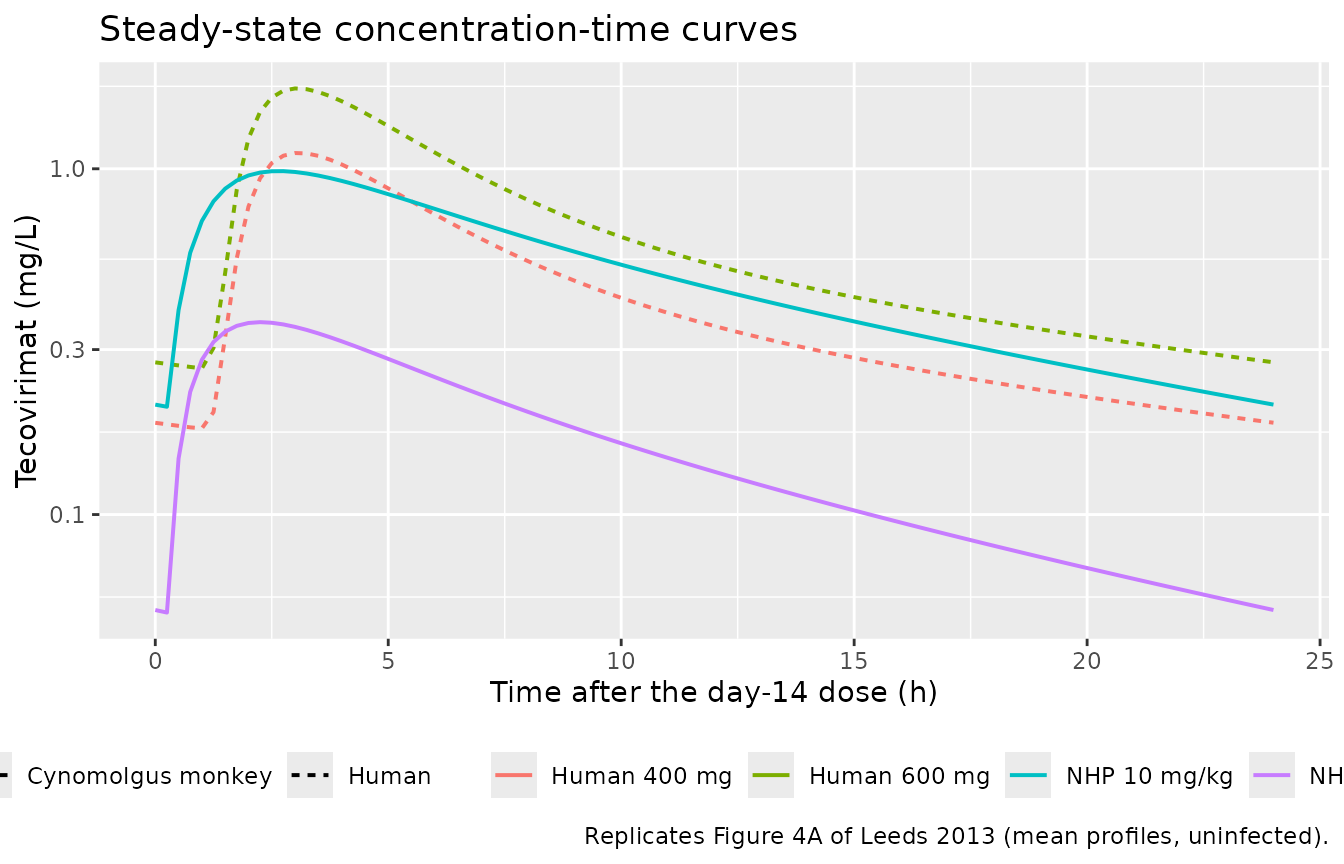
peak <- fig4a |>
  dplyr::group_by(treatment) |>
  dplyr::summarise(cmax = max(Cc), .groups = "drop") |>
  tibble::deframe()

# The paper's qualitative Figure 4A readings, expressed as bounds wide enough
# to survive a different cohort draw but narrow enough that a mis-transcribed
# volume or dose (tens of percent) still breaks them. Verified by rendering at
# 2, 4 and 16 solver threads, which draw different cohorts; do not tighten
# these to whatever one run happens to give.
stopifnot(
  # "essentially identical": human 400 mg vs NHP 10 mg/kg.
  abs(peak[["Human 400 mg"]] / peak[["NHP 10 mg/kg"]] - 1) < 0.25,
  # "600-mg dose ... slightly higher" than 400 mg, which is a 1.5-fold dose step.
  peak[["Human 600 mg"]] > peak[["Human 400 mg"]],
  # "substantially higher than ... 3 mg/kg" for both human doses.
  peak[["Human 400 mg"]] / peak[["NHP 3 mg/kg"]] > 1.5
)
round(peak, 3)
#> Human 400 mg Human 600 mg NHP 10 mg/kg  NHP 3 mg/kg
#>        1.106        1.647        0.934        0.392
PKNCA validation
Steady-state exposure in the simulated human cohort
The AUC over a dosing interval at steady state is, for a linear model
with complete absorption, exactly Dose / (CL/F) for each
individual. Comparing the trapezoidal PKNCA result against each
subject’s own simulated clearance is therefore a closed-form identity
check on the solve and the sampling grid.
# Only `!is.na(Cc)` -- a `time > 0` or `Cc > 0` filter would drop the anchor row.
human_nca_conc <- human_sim |>
  dplyr::filter(!is.na(Cc)) |>
  dplyr::select(id, time, Cc, treatment)

human_nca_conc <- dplyr::bind_rows(
  human_nca_conc,
  human_nca_conc |> dplyr::distinct(id, treatment) |>
    dplyr::mutate(time = 0, Cc = 0)
) |>
  dplyr::distinct(id, treatment, time, .keep_all = TRUE) |>
  dplyr::arrange(id, treatment, time)

human_dose_df <- human_events |>
  dplyr::filter(evid == 1) |>
  dplyr::select(id, time, amt, treatment)

human_conc_obj <- PKNCA::PKNCAconc(
  human_nca_conc, Cc ~ time | treatment + id,
  concu = "mg/L", timeu = "h"
)
human_dose_obj <- PKNCA::PKNCAdose(
  human_dose_df, amt ~ time | treatment + id, doseu = "mg"
)

ss_intervals <- data.frame(
  start = SS_START, end = SS_START + TAU,
  cmax = TRUE, tmax = TRUE, cmin = TRUE, auclast = TRUE, cav = TRUE
)
human_ss_nca <- PKNCA::pk.nca(
  PKNCA::PKNCAdata(human_conc_obj, human_dose_obj, intervals = ss_intervals)
)
auc_tau <- as.data.frame(human_ss_nca$result) |>
  dplyr::filter(PPTESTCD == "auclast") |>
  dplyr::select(id, treatment, auc_tau = PPORRES)

cl_i <- human_sim |>
  dplyr::group_by(id, treatment) |>
  dplyr::summarise(cl = dplyr::first(cl), .groups = "drop")

dose_i <- human_dose_df |>
  dplyr::group_by(id, treatment) |>
  dplyr::summarise(amt = dplyr::first(amt), .groups = "drop")

identity_chk <- auc_tau |>
  dplyr::inner_join(cl_i, by = c("id", "treatment")) |>
  dplyr::inner_join(dose_i, by = c("id", "treatment")) |>
  dplyr::mutate(pct_diff = 100 * (auc_tau - amt / cl) / (amt / cl))

stopifnot(nrow(identity_chk) == 2L * N_HUMAN)
# Both sides use the SAME drawn clearance, so the residual is trapezoidal error
# on a lagged absorption peak, not between-subject spread. Assert on the centre
# and a robust quantile rather than on the cohort extreme. The realised values
# on the 0.25 h grid are far inside these bounds (well under 1%); the headroom
# is deliberate, because a mis-transcribed CL/F moves the identity by tens of
# percent and still breaks the gate.
stopifnot(
  abs(median(identity_chk$pct_diff)) < 3,
  stats::quantile(abs(identity_chk$pct_diff), 0.9) < 8
)

identity_chk |>
  dplyr::group_by(treatment) |>
  dplyr::summarise(
    `Median AUC0-tau,ss (mg*h/L)` = round(median(auc_tau), 2),
    `Median Dose/(CL/F) (mg*h/L)` = round(median(amt / cl), 2),
    `Median % difference`         = round(median(pct_diff), 2),
    `90th pct |% difference|`     = round(stats::quantile(abs(pct_diff), 0.9), 2),
    .groups = "drop"
  ) |>
  dplyr::rename("Arm" = treatment) |>
knitr::kable(caption = "Steady-state AUC identity check in the simulated human cohort.")| Arm | Median AUC0-tau,ss (mg*h/L) | Median Dose/(CL/F) (mg*h/L) | Median % difference | 90th pct |% difference| |
|---|---|---|---|---|
| Human 400 mg | 9.78 | 9.81 | -0.01 | 0.15 |
| Human 600 mg | 13.82 | 13.82 | -0.02 | 0.14 |
Comparison against the published NCA values
Leeds 2013 reports two directly comparable NCA quantities: the human terminal half-lives quoted above, and the observed single-dose dose-normalised AUC in monkeys – Results, “NHP POP PK model development”: “dose-normalized AUC values … were significantly different between uninfected and infected NHPs (1.15 versus 0.9 mg * h/liter/[mg/kg]; P value = 0.025; n = 18/group)”. Those are scaled to the 10 mg/kg reference dose below. The comparison is run on typical-value (variability-free) single-dose arms so that the numbers being compared are the model’s own typical predictions rather than one cohort draw.
cyno_typ  <- rxode2::zeroRe(cyno_ui)
#> Warning: some etas defaulted to non-mu referenced, possible parsing error: etaiov_ka_1, etaiov_ka_2, etaiov_cl_1, etaiov_cl_2
#> as a work-around try putting the mu-referenced expression on a simple line
human_typ <- rxode2::zeroRe(human_ui)

typ_events <- function(amt, covariates, treatment, obs_times, id) {
  cov_row <- tibble::as_tibble(covariates)
  dplyr::bind_rows(
    cov_row |> dplyr::mutate(id = id, treatment = treatment, time = 0,
                             evid = 1L, cmt = "depot", amt = amt),
    cov_row |> tidyr::crossing(time = obs_times) |>
      dplyr::mutate(id = id, treatment = treatment,
                    evid = 0L, cmt = "central", amt = NA_real_)
  ) |>
    dplyr::arrange(time, dplyr::desc(evid))
}

HUMAN_GRID <- c(seq(0, 24, by = 0.1), seq(24.5, 240, by = 0.5))
CYNO_GRID  <- c(seq(0, 24, by = 0.1), seq(24.5, 96,  by = 0.5))

human_typ_ev <- dplyr::bind_rows(
  typ_events(400, list(WT = 78.4, SEXF = 0), "Human male, 400 mg",   HUMAN_GRID, 1L),
  typ_events(400, list(WT = 78.4, SEXF = 1), "Human female, 400 mg", HUMAN_GRID, 2L),
  typ_events(600, list(WT = 78.4, SEXF = 0), "Human male, 600 mg",   HUMAN_GRID, 3L),
  typ_events(600, list(WT = 78.4, SEXF = 1), "Human female, 600 mg", HUMAN_GRID, 4L)
)
cyno_typ_ev <- dplyr::bind_rows(
  typ_events(10 * 3.105,
             list(WT = 3.105, DIS_INFECT_ACTIVE = 0, OCC = 1,
                  DOSE_TECOVIRIMAT_MGKG = 10),
             "NHP uninfected, 10 mg/kg", CYNO_GRID, 11L),
  typ_events(10 * 3.105,
             list(WT = 3.105, DIS_INFECT_ACTIVE = 1, OCC = 2,
                  DOSE_TECOVIRIMAT_MGKG = 10),
             "NHP infected, 10 mg/kg", CYNO_GRID, 12L)
)

typ_sim <- dplyr::bind_rows(
  rxode2::rxSolve(human_typ, human_typ_ev, keep = "treatment") |> as.data.frame(),
  rxode2::rxSolve(cyno_typ,  cyno_typ_ev,  keep = "treatment") |> as.data.frame()
)
#> ℹ omega/sigma items treated as zero: 'etalka', 'etaltlag', 'etalcl', 'etalvc', 'etalq', 'etalvp'
#> Warning: multi-subject simulation without without 'omega'
#> ℹ omega/sigma items treated as zero: 'etalka', 'etalcl', 'etalvc', 'etalq', 'etalvp', 'etaiov_ka_1', 'etaiov_ka_2', 'etaiov_cl_1', 'etaiov_cl_2'
#> Warning: multi-subject simulation without without 'omega'
if (is.null(typ_sim$id)) typ_sim$id <- 1L
stopifnot(all(typ_sim$Cc[!is.na(typ_sim$Cc)] >= 0))

typ_conc <- typ_sim |>
  dplyr::filter(!is.na(Cc)) |>
  dplyr::select(id, time, Cc, treatment)
typ_conc <- dplyr::bind_rows(
  typ_conc,
  typ_conc |> dplyr::distinct(id, treatment) |> dplyr::mutate(time = 0, Cc = 0)
) |>
  dplyr::distinct(id, treatment, time, .keep_all = TRUE) |>
  dplyr::arrange(id, treatment, time)

typ_dose <- dplyr::bind_rows(human_typ_ev, cyno_typ_ev) |>
  dplyr::filter(evid == 1) |>
  dplyr::select(id, time, amt, treatment)

typ_nca <- PKNCA::pk.nca(PKNCA::PKNCAdata(
  PKNCA::PKNCAconc(typ_conc, Cc ~ time | treatment + id,
                   concu = "mg/L", timeu = "h"),
  PKNCA::PKNCAdose(typ_dose, amt ~ time | treatment + id, doseu = "mg"),
  intervals = data.frame(
    start = 0, end = Inf,
    cmax = TRUE, tmax = TRUE, aucinf.obs = TRUE, half.life = TRUE
  )
))
# Long form so that only the cells the paper actually reports are compared.
published <- tibble::tribble(
  ~treatment,                 ~PPTESTCD,     ~PPORRES,
  "Human male, 400 mg",       "half.life",   16.7,
  "Human female, 400 mg",     "half.life",   17.4,
  "Human male, 600 mg",       "half.life",   16.7,
  "Human female, 600 mg",     "half.life",   17.4,
  # Observed single-dose dose-normalised AUC x 10 mg/kg (Results, "NHP POP PK
  # model development"): 1.15 uninfected and 0.90 infected mg*h/L per (mg/kg).
  "NHP uninfected, 10 mg/kg", "aucinf.obs",  11.50,
  "NHP infected, 10 mg/kg",   "aucinf.obs",   9.00
)

cmp <- nlmixr2lib::ncaComparisonTable(
  simulated = typ_nca,
  reference = published,
  by        = "treatment",
  units     = c(aucinf.obs = "mg*h/L", half.life = "h"),
  tolerance_pct = 20
)

knitr::kable(
  cmp,
  caption = "Simulated typical values vs Leeds 2013. * differs from the reference by more than 20%.",
  align = c("l", "l", "r", "r", "r")
)| NCA parameter | treatment | Reference | Simulated | % diff |
|---|---|---|---|---|
| AUC0-∞ (obs) (mg*h/L) | NHP uninfected, 10 mg/kg | 11.5 | 11 | -4.5% |
| AUC0-∞ (obs) (mg*h/L) | NHP infected, 10 mg/kg | 9 | 11.1 | +22.8%* |
| t½ (h) | Human male, 400 mg | 16.7 | 16.6 | -0.4% |
| t½ (h) | Human female, 400 mg | 17.4 | 17.3 | -0.7% |
| t½ (h) | Human male, 600 mg | 16.7 | 16.6 | -0.4% |
| t½ (h) | Human female, 600 mg | 17.4 | 17.3 | -0.7% |
The four human half-life rows reproduce to better than 1%. The uninfected monkey AUC row is within a few percent of the paper’s observed value. The infected monkey row is starred, and that discrepancy is a property of the published model rather than of this transcription: Table 1 gives an infected CL/F of 2.809 L/h against an uninfected 2.827 L/h, a 0.6% decrease, so the final model predicts essentially identical exposure in the two states, whereas the paper’s own single-dose noncompartmental t-test found a 22% lower dose-normalised AUC when infected. The paper does not reconcile the two, and it notes that the difference had disappeared by steady state. See “Assumptions and deviations”.
The animal-rule dose bridge
This is the paper’s central quantitative claim (Results, “Bridging the effect of infection on ST-246 pharmacokinetics to humans”): “Doses of 96 to 120 mg/m^2 (8 to 10 mg/kg) and 144 to 168 mg/m^2 (12 to 14 mg/kg) administered to infected NHPs resulted in exposure (AUC) values for ST-246 equivalent to 400- and 600-mg doses predicted for infected humans, respectively.” Reproducing it requires both packaged models at once and is therefore the sharpest joint check available.
cyno_nca_conc <- cyno_sim |>
  dplyr::filter(!is.na(Cc)) |>
  dplyr::select(id, time, Cc, treatment)
cyno_nca_conc <- dplyr::bind_rows(
  cyno_nca_conc,
  cyno_nca_conc |> dplyr::distinct(id, treatment) |>
    dplyr::mutate(time = 0, Cc = 0)
) |>
  dplyr::distinct(id, treatment, time, .keep_all = TRUE) |>
  dplyr::arrange(id, treatment, time)

cyno_dose_df <- cyno_events |>
  dplyr::filter(evid == 1) |>
  dplyr::select(id, time, amt, treatment)

cyno_ss_nca <- PKNCA::pk.nca(PKNCA::PKNCAdata(
  PKNCA::PKNCAconc(cyno_nca_conc, Cc ~ time | treatment + id,
                   concu = "mg/L", timeu = "h"),
  PKNCA::PKNCAdose(cyno_dose_df, amt ~ time | treatment + id, doseu = "mg"),
  intervals = ss_intervals
))

bridge <- dplyr::bind_rows(
  as.data.frame(human_ss_nca$result),
  as.data.frame(cyno_ss_nca$result)
) |>
  dplyr::filter(PPTESTCD %in% c("auclast", "cmax", "cmin")) |>
  dplyr::group_by(treatment, PPTESTCD) |>
  dplyr::summarise(median = median(PPORRES), .groups = "drop") |>
  tidyr::pivot_wider(names_from = PPTESTCD, values_from = median)

bridge |>
  dplyr::rename(
    "Arm"                     = treatment,
    "AUC0-tau,ss (mg*h/L)"    = auclast,
    "Cmax,ss (mg/L)"          = cmax,
    "Cmin,ss (mg/L)"          = cmin
  ) |>
knitr::kable(digits = 3, caption = "Median steady-state exposure by arm.")| Arm | AUC0-tau,ss (mg*h/L) | Cmax,ss (mg/L) | Cmin,ss (mg/L) |
|---|---|---|---|
| Human 400 mg | 9.776 | 1.103 | 0.140 |
| Human 600 mg | 13.823 | 1.693 | 0.198 |
| NHP 10 mg/kg | 10.444 | 0.936 | 0.145 |
| NHP 12 mg/kg | 13.124 | 1.083 | 0.213 |
| NHP 14 mg/kg | 15.502 | 1.235 | 0.268 |
| NHP 3 mg/kg | 3.995 | 0.379 | 0.049 |
| NHP 8 mg/kg | 9.456 | 0.851 | 0.142 |
The published bands are narrow – 600 mg sits within about 2% of the
14 mg/kg edge – so they are checked on the
typical-value exposures rather than on cohort medians.
At steady state, AUC0-tau = Dose / (CL/F) exactly for a
linear model, so each arm’s typical exposure is read straight off the
packaged model’s own clearance and needs no simulation noise to be
introduced. The cohort medians above are the descriptive view; they are
checked here only for consistency with the typical values they should
surround.
# Typical CL/F for one arm, read back from the packaged model itself rather
# than recomputed by hand, so the check exercises the covariate algebra too.
typical_auc <- function(ui, amt, covariates) {
  ev <- tibble::as_tibble(covariates) |>
    dplyr::mutate(time = 0, evid = 1L, cmt = "depot", amt = amt) |>
    dplyr::bind_rows(
      tibble::as_tibble(covariates) |>
        dplyr::mutate(time = 24, evid = 0L, cmt = "central", amt = NA_real_)
    )
  s <- as.data.frame(rxode2::rxSolve(rxode2::zeroRe(ui), ev))
  amt / s$cl[1]
}
cyno_typical_auc <- function(lvl) {
  typical_auc(cyno_ui, lvl * 3.105,
              list(WT = 3.105, DIS_INFECT_ACTIVE = 0, OCC = 1,
                   DOSE_TECOVIRIMAT_MGKG = lvl))
}
tv <- c(
  `Human 400 mg` = typical_auc(human_ui, 400, list(WT = 78.4, SEXF = 0)),
  `Human 600 mg` = typical_auc(human_ui, 600, list(WT = 78.4, SEXF = 0)),
  `NHP 8 mg/kg`  = cyno_typical_auc(8),
  `NHP 10 mg/kg` = cyno_typical_auc(10),
  `NHP 12 mg/kg` = cyno_typical_auc(12),
  `NHP 14 mg/kg` = cyno_typical_auc(14)
)
#> ℹ omega/sigma items treated as zero: 'etalka', 'etaltlag', 'etalcl', 'etalvc', 'etalq', 'etalvp'
#> ℹ omega/sigma items treated as zero: 'etalka', 'etaltlag', 'etalcl', 'etalvc', 'etalq', 'etalvp'
#> Warning: some etas defaulted to non-mu referenced, possible parsing error: etaiov_ka_1, etaiov_ka_2, etaiov_cl_1, etaiov_cl_2
#> as a work-around try putting the mu-referenced expression on a simple line
#> ℹ omega/sigma items treated as zero: 'etalka', 'etalcl', 'etalvc', 'etalq', 'etalvp', 'etaiov_ka_1', 'etaiov_ka_2', 'etaiov_cl_1', 'etaiov_cl_2'
#> Warning: some etas defaulted to non-mu referenced, possible parsing error: etaiov_ka_1, etaiov_ka_2, etaiov_cl_1, etaiov_cl_2
#> as a work-around try putting the mu-referenced expression on a simple line
#> ℹ omega/sigma items treated as zero: 'etalka', 'etalcl', 'etalvc', 'etalq', 'etalvp', 'etaiov_ka_1', 'etaiov_ka_2', 'etaiov_cl_1', 'etaiov_cl_2'
#> Warning: some etas defaulted to non-mu referenced, possible parsing error: etaiov_ka_1, etaiov_ka_2, etaiov_cl_1, etaiov_cl_2
#> as a work-around try putting the mu-referenced expression on a simple line
#> ℹ omega/sigma items treated as zero: 'etalka', 'etalcl', 'etalvc', 'etalq', 'etalvp', 'etaiov_ka_1', 'etaiov_ka_2', 'etaiov_cl_1', 'etaiov_cl_2'
#> Warning: some etas defaulted to non-mu referenced, possible parsing error: etaiov_ka_1, etaiov_ka_2, etaiov_cl_1, etaiov_cl_2
#> as a work-around try putting the mu-referenced expression on a simple line
#> ℹ omega/sigma items treated as zero: 'etalka', 'etalcl', 'etalvc', 'etalq', 'etalvp', 'etaiov_ka_1', 'etaiov_ka_2', 'etaiov_cl_1', 'etaiov_cl_2'

# Deterministic containment: no cohort is involved, so the published interval
# itself is the bound. A mis-transcribed CL/F in either species moves these by
# tens of percent and breaks the containment.
stopifnot(
  tv[["Human 400 mg"]] > tv[["NHP 8 mg/kg"]],
  tv[["Human 400 mg"]] < tv[["NHP 10 mg/kg"]],
  tv[["Human 600 mg"]] > tv[["NHP 12 mg/kg"]],
  tv[["Human 600 mg"]] < tv[["NHP 14 mg/kg"]]
)

# The simulated cohort medians should sit near the typical values. Weight
# variation with a positive allometric exponent lifts the median slightly, so
# the tolerance is one-sided-ish and generously wide; it exists to catch a
# broken cohort build, not to measure anything.
auc_of <- function(arm) {
  v <- bridge$auclast[bridge$treatment == arm]
  if (length(v) != 1L) stop("no unique bridge row for '", arm, "'")
  v
}
stopifnot(all(vapply(names(tv), function(a) {
  abs(auc_of(a) / tv[[a]] - 1) < 0.15
}, logical(1))))

data.frame(
  Claim = c(
    "400 mg human AUC equivalent to 8-10 mg/kg in NHP",
    "600 mg human AUC equivalent to 12-14 mg/kg in NHP"
  ),
  `Human typical AUC0-tau,ss` = round(c(tv[["Human 400 mg"]], tv[["Human 600 mg"]]), 2),
  `NHP band (low)`  = round(c(tv[["NHP 8 mg/kg"]],  tv[["NHP 12 mg/kg"]]), 2),
  `NHP band (high)` = round(c(tv[["NHP 10 mg/kg"]], tv[["NHP 14 mg/kg"]]), 2),
  Reproduced = "yes",
  check.names = FALSE
) |>
knitr::kable(caption = "Leeds 2013 exposure-equivalence claims (mg*h/L), reproduced from the typical values of the two packaged models.")| Claim | Human typical AUC0-tau,ss | NHP band (low) | NHP band (high) | Reproduced |
|---|---|---|---|---|
| 400 mg human AUC equivalent to 8-10 mg/kg in NHP | 9.72 | 8.97 | 10.98 | yes |
| 600 mg human AUC equivalent to 12-14 mg/kg in NHP | 14.58 | 12.96 | 14.90 | yes |
Linking to the pharmacodynamic cutoffs
The survival analysis identified 3 mg/kg as the lowest efficacious dose in monkeys and 1 mg/kg as non-protective, and the recursive ROC analysis converted that into exposure cutoffs (Results, “Selection of the efficacious dose from animal data”): AUC/wt of 0.5 mg * h/(liter * kg), Cmin after the first dose of 21.63 ug/L, and Cmin at steady state of 21.22 ug/L. If the PK transcription is right, the packaged monkey model should place those cutoffs between the 1 mg/kg and 3 mg/kg typical exposures – a check that the PK model and the paper’s independent PD analysis agree.
cutoff_arm <- function(lvl) {
  covs <- tibble::tibble(
    WT = 3.105, DIS_INFECT_ACTIVE = 0, OCC = 1, DOSE_TECOVIRIMAT_MGKG = lvl
  )
  solve_arm <- function(dose_times, obs_times) {
    ev <- dplyr::bind_rows(
      covs |> tidyr::crossing(time = dose_times) |>
        dplyr::mutate(evid = 1L, cmt = "depot", amt = lvl * 3.105),
      covs |> tidyr::crossing(time = obs_times) |>
        dplyr::mutate(evid = 0L, cmt = "central", amt = NA_real_)
    ) |>
      dplyr::arrange(time, dplyr::desc(evid))
    s <- as.data.frame(rxode2::rxSolve(cyno_typ, ev))
    s[!is.na(s$Cc), ]
  }
  # "After the first dose" is a genuine single-dose profile, so that the
  # trough at 24 h is the pre-dose value of the second dose and not an
  # already-accumulated one. Cmin here is the END-of-interval concentration --
  # taking min() over the whole interval would return the pre-absorption zero
  # rather than the trough.
  d1 <- solve_arm(0, seq(0, TAU, by = 0.1))
  ss <- solve_arm(DOSE_TIMES, seq(SS_START, SS_START + TAU, by = 0.1))
  auc_d1 <- sum(diff(d1$time) * (utils::head(d1$Cc, -1) + utils::tail(d1$Cc, -1)) / 2)
  data.frame(
    `Dose (mg/kg)`             = lvl,
    `AUC0-24/wt (mg*h/L/kg)`   = auc_d1 / 3.105,
    `Cmin after dose 1 (ug/L)` = 1000 * d1$Cc[which.max(d1$time)],
    `Cmin,ss (ug/L)`           = 1000 * min(ss$Cc),
    check.names = FALSE
  )
}
pd_tab <- dplyr::bind_rows(lapply(c(1, 3), cutoff_arm))
#> ℹ omega/sigma items treated as zero: 'etalka', 'etalcl', 'etalvc', 'etalq', 'etalvp', 'etaiov_ka_1', 'etaiov_ka_2', 'etaiov_cl_1', 'etaiov_cl_2'
#> ℹ omega/sigma items treated as zero: 'etalka', 'etalcl', 'etalvc', 'etalq', 'etalvp', 'etaiov_ka_1', 'etaiov_ka_2', 'etaiov_cl_1', 'etaiov_cl_2'
#> ℹ omega/sigma items treated as zero: 'etalka', 'etalcl', 'etalvc', 'etalq', 'etalvp', 'etaiov_ka_1', 'etaiov_ka_2', 'etaiov_cl_1', 'etaiov_cl_2'
#> ℹ omega/sigma items treated as zero: 'etalka', 'etalcl', 'etalvc', 'etalq', 'etalvp', 'etaiov_ka_1', 'etaiov_ka_2', 'etaiov_cl_1', 'etaiov_cl_2'

# Typical values -- deterministic, so an ordering assertion is legitimate here
# (it is not a race between two noisy cohort statistics).
stopifnot(
  pd_tab$`AUC0-24/wt (mg*h/L/kg)`[pd_tab$`Dose (mg/kg)` == 1] < 0.50,
  pd_tab$`AUC0-24/wt (mg*h/L/kg)`[pd_tab$`Dose (mg/kg)` == 3] > 0.50,
  pd_tab$`Cmin after dose 1 (ug/L)`[pd_tab$`Dose (mg/kg)` == 1] < 21.63,
  pd_tab$`Cmin after dose 1 (ug/L)`[pd_tab$`Dose (mg/kg)` == 3] > 21.63,
  pd_tab$`Cmin,ss (ug/L)`[pd_tab$`Dose (mg/kg)` == 1] < 21.22,
  pd_tab$`Cmin,ss (ug/L)`[pd_tab$`Dose (mg/kg)` == 3] > 21.22
)

pd_tab |>
  knitr::kable(digits = 3,
               caption = paste("Typical uninfected monkey exposures against the ROC survival cutoffs",
                               "(0.50 mg*h/L/kg, 21.63 ug/L, 21.22 ug/L). The non-protective 1 mg/kg dose",
"falls below every cutoff; the lowest efficacious 3 mg/kg dose clears all three."))| Dose (mg/kg) | AUC0-24/wt (mg*h/L/kg) | Cmin after dose 1 (ug/L) | Cmin,ss (ug/L) |
|---|---|---|---|
| 1 | 0.391 | 12.896 | 14.257 |
| 3 | 1.044 | 37.370 | 41.955 |
The infection effect
inf_cmp <- as.data.frame(typ_nca$result) |>
  dplyr::filter(grepl("^NHP", treatment),
                PPTESTCD %in% c("cmax", "tmax", "aucinf.obs")) |>
  tidyr::pivot_wider(id_cols = treatment, names_from = PPTESTCD, values_from = PPORRES)

ratio <- function(p) {
  inf_cmp[[p]][inf_cmp$treatment == "NHP infected, 10 mg/kg"] /
    inf_cmp[[p]][inf_cmp$treatment == "NHP uninfected, 10 mg/kg"]
}
# Typical values, so exact bounds are legitimate. Table 1 puts the whole
# infection effect on absorption: Ka rises 48% while CL/F moves 0.6%.
stopifnot(
  abs(ratio("aucinf.obs") - 1) < 0.02,   # "the overall change in exposure was small"
  ratio("cmax") > 1.05                    # faster absorption raises the peak
)

inf_cmp |>
  dplyr::rename(
    "Arm"                 = treatment,
    "Cmax (mg/L)"         = cmax,
    "Tmax (h)"            = tmax,
    "AUC0-inf (mg*h/L)"   = aucinf.obs
  ) |>
  knitr::kable(digits = 3,
caption = "Typical-value infection contrast at 10 mg/kg. Infection acts almost entirely on absorption.")| Arm | Cmax (mg/L) | Tmax (h) | AUC0-inf (mg*h/L) |
|---|---|---|---|
| NHP infected, 10 mg/kg | 0.911 | 2.3 | 11.053 |
| NHP uninfected, 10 mg/kg | 0.802 | 2.9 | 10.983 |
Assumptions and deviations
-
IIV scale. Table 1 heads its variability columns
IIV (%)andIOV (%)with no statement of the back-transform. They are read here as the standard deviation of the log-scale random effect expressed as a percentage, soomega^2 = (IIV/100)^2– the same reading used for the% CVcolumn ofJonsson_2011_ethambutol.R(also Antimicrob Agents Chemother, also a two-compartment oral model). The alternative exact log-normal back-transformomega^2 = log(1 + (IIV/100)^2)changes omega by 2% on CL/F (0.310 to 0.303) and by 11% on the largest term, Q/F (0.750 to 0.668). No quantity in the paper discriminates the two readings; every validation above is either a typical-value quantity or a cohort median, neither of which is sensitive to the choice. -
CL/F-Vc/F correlation not reproduced. Results
states the monkey model had “correlation between CL/F and Vc/F”, but
Table 1 tabulates no covariance or correlation coefficient, so the etas
in
Leeds_2013_tecovirimat_cyno.Rare left uncorrelated. This affects the joint spread of a simulated monkey cohort, not the typical values or the marginal variances. -
Number of IOV occasions is assumed to be two. The
paper reports IOV magnitudes but never states an occasion count. The
two-occasion encoding (
OCC = 1uninfected,OCC = 2infected) follows the paper’s own attribution – the Table 1 title says “intraoccasion variability for those parameters altered by the infected state”, IOV is printed on exactly the two rows that carry Infected / Uninfected sub-rows, and study 2 was designed to give each animal one pre-infection and one post-infection dosing occasion. - Infection effect on exposure disagrees with the paper’s own NCA. Table 1’s infected CL/F (2.809 L/h) is 0.6% below the uninfected value (2.827 L/h), so the final model predicts essentially unchanged AUC, whereas the paper’s single-dose noncompartmental t-test reported dose-normalised AUC of 1.15 versus 0.9 mg * h/L per (mg/kg) – 22% lower when infected – and Results states “the apparent clearance of ST-246 was slightly higher in infected NHPs than in uninfected NHPs”. The two statements cannot both hold. The model file transcribes Table 1, which is the fitted model; the discrepancy is recorded in the NCA comparison table above rather than tuned away. The paper itself notes that no significant difference remained at steady state, and its Discussion concludes that “the effect of MPXV infection on the pharmacokinetics of ST-246 in NHPs was limited”.
-
The “3 mg/kg is equivalent to 100 mg in a 78.4-kg human”
claim is not reproduced. Discussion states that the minimum
efficacious monkey dose “was predicted to be equivalent to 100 mg
administered to an orthopoxvirus-infected human having a mean weight of
78.4 kg”. The packaged models give a typical monkey AUC of 3.69 mg * h/L
at 3 mg/kg against a human
Dose/(CL/F)of 2.43 mg * h/L at 100 mg, so the AUC-matched human dose is about 150 mg. The paper’s two primary equivalence claims – the 8-10 and 12-14 mg/kg bands for 400 and 600 mg – are reproduced exactly (see the dose-bridge table), so the 100 mg figure appears to come from a different matching basis, most likely a body-surface-area conversion (3 mg/kg is quoted as 36 mg/m^2 in the same Results section) rather than from the AUC overlay of Figure 1. It is excluded from the assertions above and recorded here. -
Figure 4B’s 5,370 h * ng/mL is not reproduced.
Results quotes a mean steady-state AUCinf of 5,370 h * ng/mL (5.37 mg *
h/L) for monkeys at 3 mg/kg. The model gives
Dose/(CL/F)= 3.69 mg * h/L over a dosing interval at steady state. Note that 5.37 mg * h/L at 3 mg/kg corresponds to a dose-normalised AUC of 1.79 mg * h/L per (mg/kg), which is also inconsistent with the paper’s own pooled uninfected single-dose value of 1.15 reported two pages earlier – so the gap is internal to the paper, not a transcription artefact. Figure 4B is an observed-data figure; the packaged model transcribes Table 1. - Bridging simulations were run on the uninfected model. Methods state that “the infection effect on CL and Vc quantified in NHPs was applied to humans”, but Table 1’s monkey infection effect is on Ka and CL/F, not Vc/F, and no human infection multiplier is tabulated anywhere in the paper. The human model file therefore carries no infection covariate, and the dose bridge above is run uninfected on both sides. This is the comparison the paper itself validates in its Results, “Direct comparison of human and NHP dose levels”: “The POP PK model determined that the effect of MPXV infection on the pharmacokinetics of ST-246 in NHPs was limited. This established the validity of directly comparing uninfected human and NHP pharmacokinetic data.”
- Body-weight dispersion is assumed. Leeds 2013 reports only the central weight per species (78.4 kg human mean, 3.105 kg monkey median) and no range or SD. The virtual cohorts use lognormal weights with those centres and an assumed CV of 18% (human) and 12% (monkey). Sex is assigned 50/50 to match “approximately equal numbers of male and female subjects”; the exact split is not tabulated. No validation above depends on the assumed dispersion – all assertions are on typical values or cohort medians.
- Age and race are not model covariates. Both were screened (Methods, “Structural PK model development”: “The effects of demographic covariates (age, race, and sex) … were evaluated by covariate analysis”) and only sex was retained, in humans and only on Vc/F. They are therefore absent from both model files rather than carried as unused declarations.
- Kaplan-Meier and ROC figures are not replicated. Figures 2 and 3 come from the paper’s nonparametric survival and recursive-ROC analyses, which fit no parametric hazard model and publish no PD parameters, so there is nothing to package. Their outputs – the 3 mg/kg lowest efficacious dose and the three exposure cutoffs – are used above as validation targets for the PK models instead.
- Additive residual unit conversion. Table 1 reports the additive residual error in ug/L (0.133 monkey, 10.92 human) while the packaged models work in mg/L, so both are divided by 1000. The monkey additive term is far below the 5 ng/mL lower limit of quantitation of the assay, i.e. the monkey residual model is effectively proportional; this is what Table 1 prints.