Morphine brain-ECF PK and P-gp DDIs at the BBB with LeiCNS-PK3.0 (Gulave 2025)
Source:vignettes/articles/Gulave_2025_morphine_pbpk.Rmd
Gulave_2025_morphine_pbpk.RmdModel and source
Gulave B, Lesmana A, de Lange ECM, van Hasselt JGC. Do P-glycoprotein-mediated drug-drug interactions at the blood-brain barrier impact morphine brain distribution? J Pharmacokinet Pharmacodyn 2025;52(1):10. doi:10.1007/s10928-024-09957-0.
The paper asks whether clinically used P-glycoprotein (P-gp) inhibitors can raise unbound morphine concentrations in human brain extracellular fluid (brain ECF) by blocking P-gp at the blood-brain barrier (BBB). It answers with simulations of the human LeiCNS-PK3.0 CNS physiologically-based PK model, extended for morphine’s nonlinear BBB transport. No clinical data were fitted.
The model is assembled from three earlier publications, all cited by the paper:
- CNS structure and human physiology: LeiCNS-PK3.0, Saleh et al. 2021 (doi:10.1007/s10928-021-09768-7), Supplementary Table 2 and the supplementary equations for the barrier clearances and asymmetry factors.
- Morphine extension: Gulave et al. 2023 (doi:10.1016/j.ejps.2023.106482), which introduced the concentration-dependent Kp,uu,BBB and the rat-to-human translation factor fAF_BBB.
-
Plasma input: the one-compartment morphine
population PK model of Oosten et al. 2017 (doi:10.1007/s40262-016-0471-7),
also packaged as
Oosten_2017_morphine.
mod <- readModelDb("Gulave_2025_morphine_pbpk")
mod_typ <- rxode2::zeroRe(mod)
#> ℹ parameter labels from comments will be replaced by 'label()'
How the pieces fit
- Plasma is a forcing function: the Oosten 2017 one-compartment model for a 70 kg adult (CL 91.9 L/h, V 278 L). Brain uptake does not deplete it.
-
Nonlinear BBB transport. The extent of BBB
transport depends on the instantaneous unbound plasma concentration
Cu(ng/mL), Table 1:Kp,uu,BBB = 14.543 / (1 + (Cu / 5.902)^0.895). It is above 1 (net influx) at low concentrations and falls below 1 (net efflux) above about 109 ng/mL. - Asymmetry factors. As in every LeiCNS-PK3.0 model, active transport is an asymmetry factor (AF) on the transcellular clearance. When Kp,uu,BBB >= 1 the efflux AF is 1 and the influx AF is back-calculated from Kp,uu,BBB; when Kp,uu,BBB < 1 the influx AF is 1 and the efflux AF is back-calculated (Supplementary Eqs. 3-4). Because the Kp,uu function was derived in rats, the back-calculated BBB factor is multiplied by fAF_BBB = 0.218, the human-to-rat ratio of BBB P-gp protein expression (4.21 vs 19.28 fmol/ug).
-
The DDI. A P-gp inhibitor divides the BBB
transcellular efflux clearance by
1 + fu,p * [I] / Ki(Rowland-Matin, Eqs. 2-4). The ratio is the covariateINH_PGP_RATIO; 0 means no inhibitor.
Population
There is no study population. The paper simulates 2000 virtual adults, each a 70 kg individual whose plasma clearance and volume vary with the Oosten 2017 interindividual variances (0.222 and 0.747 on the log scale; Table 1). Morphine is given as 10 mg IV every 4 h for 7 days (0.1-0.2 mg/kg every 4 h at 70 kg), and, in the sensitivity analyses, 50 and 100 mg every 4 h. The 34 inhibitors (33 clinical P-gp inhibitors and the positive control tariquidar) are dosed at their clinical maintenance regimens and enter as their steady-state plasma concentrations (Supplementary Table 1). This vignette uses 200 virtual subjects per arm.
Source trace
| Item | Value | Source |
|---|---|---|
| Plasma clearance CL | 91.9 L/h (1531.67 mL/min) | Table 1 (Oosten 2017); mL/min form in Gulave 2023 Table 1 |
| Plasma volume V | 278 L | Table 1 |
| IIV on CL / V (variance) | 0.222 / 0.747 | Table 1 |
| Proportional residual error (variance) | 0.286 | Table 1 |
| Molecular weight, logP, pKa, pKb | 285.34, 0.99, 10.26, 9.12 | Table 1 (DrugBank) |
| Unbound fraction in plasma | 0.65 | Table 1 |
| Kp,uu,BBB function | (14.543 Cu^-0.895) / (5.902^-0.895 + Cu^-0.895) | Table 1, footnote c |
| fAF_BBB | 0.21815 | Table 1, footnote b; Methods (4.21 / 19.28 fmol/ug) |
| AF_BBB scaling by fAF_BBB | back-calculated AF x fAF_BBB | Gulave 2023 Methods 2.2; Fig. 4 of this paper |
| DDI term | QtBBB x AFeBBB / (1 + fu,p [I] / Ki) | Eqs. 2-4 |
| Inhibitor fu,p, Css, Ki/IC50, DDI | 34 inhibitors | Supplementary Table 1 |
| Qp = Daq / width x SAp; Qt = 0.5 P0 SAt | - | Supplementary Eqs. 1-2; Saleh 2021 supplementary equations |
| Daq, P0 regressions | log10 Daq = -4.113 - 0.4609 log10 MW; log10 P0 = 0.939 logP - 6.21 | Saleh 2021 supplementary equations |
| AF closed forms (BBB, LV, TFV) | - | Supplementary Eqs. 3-4; Saleh 2021 supplementary equations |
| Brain volumes MV / ECF / ICF / LYS | 45 / 253 / 1000 / 12.5 mL | Saleh 2021 Suppl. table 2 |
| CSF volumes LV / TFV / CM / SAS | 20 / 3 / 1 / 116 mL | Saleh 2021 Suppl. table 2 |
| Brain phospholipid volume | 5% of 1250 mL | Saleh 2021 main text and Suppl. table 2 |
| Q_CBF / Q_ECF / Q_CSF | 689 / 0.2 / 0.42 mL/min | Saleh 2021 Suppl. table 2 |
| SA BBB / BCSFB / BCM / LYS | 150000 / 15000 / 2666520 / 1980260 cm^2 | Saleh 2021 Suppl. table 2 |
| Effective SA trans / para BBB / para BCSFB | 99.8% / 0.004% / 0.016% | Saleh 2021 Suppl. table 2 |
| Barrier widths | 0.5 um (BBB and BCSFB) | Saleh 2021 Suppl. table 2 |
| pH plasma, MV / ECF / CSF / ICF / LYS | 7.4 / 7.3 / 7.3 / 7.0 / 5.0 | Saleh 2021 Suppl. table 2 |
Simulation helpers
# Supplementary Table 1: inhibitor properties and the printed 'DDI' column,
# DDI = (fu,p * Css) / (Ki or IC50).
inhibitors <- tibble::tribble(
  ~inhibitor, ~ki_um, ~fu_p, ~css_ngml, ~ddi_printed,
  "amiodarone", 5.78, 0.04, 721.5, 7.7,
  "amisulpride", 123.5, 0.725, 691.6, 11.0,
  "amlodipine", 22, 0.02, 82.7, 0.2,
  "atorvastatin", 289, 0.02, 44.4, 0.01,
  "barnidipine", 10.6, 0.08, 18.3, 0.3,
  "bromocriptine", 3.39, 0.08, 1.3, 0.05,
  "carvedilol", 5.7, 0.02, 57.9, 0.5,
  "chlorpromazine", 0.6, 0.05, 1054, 275.5,
  "clozapine", 92.78, 0.03, 412.5, 0.4,
  "desloratadine", 43, 0.15, 1.7, 0.02,
  "diltiazem", 56.4, 0.25, 555.6, 5.9,
  "domperidone", 45.64, 0.08, 11.1, 0.05,
  "felodipine", 29.3, 0.01, 8.7, 0.01,
  "fentanyl", 6.5, 0.175, 3.8, 0.3,
  "fluoxetine", 115.5, 0.055, 68.9, 0.1,
  "flupentixol", 18.32, 0.01, 12, 0.02,
  "fluvoxamine", 146.7, 0.2, 283.3, 1.2,
  "haloperidol", 0.2, 0.1, 7.6, 10.2,
  "lansoprazole", 62.8, 0.03, 39.7, 0.05,
  "loratadine", 11.4, 0.02, 0.5, 0.00,
  "metoprolol", 200, 0.1, 138.9, 0.3,
  "nifedipine", 472, 0.05, 72.5, 0.02,
  "omeprazole", 17.7, 0.05, 50.5, 0.4,
  "pantoprazole", 17.9, 0.02, 132.3, 0.4,
  "paroxetine", 29.8, 0.05, 115.7, 0.6,
  "perphenazine", 15.45, 0.05, 10, 0.08,
  "propranolol", 48, 0.1, 274.3, 2.2,
  "quetiapine", 12.8, 0.17, 125, 4.3,
  "quinidine", 12, 0.14, 3968.2, 142.7,
  "risperidone", 25.9, 0.1, 3.3, 0.03,
  "sertraline", 31.8, 0.02, 216.4, 0.4,
  "simvastatin", 30.6, 0.05, 18.9, 0.07,
  "tariquidar", 0.23, 0.005, 500.8, 16.8,
  "verapamil", 0.3, 0.1, 498, 365.1
)

# The printed DDI column equals fu,p * Css[nM] / Ki[uM] (Css converted with
# the inhibitor molecular weight), 1000-fold the dimensionless ratio -- see
# Assumptions and deviations. The published simulations used the printed
# values, so the figure replications below do too. Loratadine prints 0.00 at
# two decimals; on the same scale it is 0.02 * (0.5 / 382.9 * 1000) / 11.4 =
# 0.00229 (molecular weight 382.9 g/mol, not given in the paper), needed as a
# non-zero base for the Figure 3 perturbations.
loratadine_ddi <- 0.02 * (0.5 / 382.9 * 1000) / 11.4

dose_ng <- function(mg) mg * 1e6
tau <- 240                      # every 4 h (min)
n_doses <- 6 * 7                # 7 days
day7 <- c(6 * 1440, 7 * 1440)   # last 24 h: the paper's AUC window

# Event table for one regimen; observation rows sample the morphine ODE states.
regimen_events <- function(mg, ids = 1L) {
  ev <- et(amt = dose_ng(mg), ii = tau, addl = n_doses - 1, cmt = "central") |>
    et(seq(day7[1], day7[2], by = 10), cmt = "brain_ecf")
  et(ev, id = ids)
}

trap_auc <- function(time, conc) sum(diff(time) * (head(conc, -1) + tail(conc, -1)) / 2)

# Typical-subject AUC of unbound brain-ECF morphine over the last 24 h.
auc_ecf_typical <- function(mg, ratio, extra = NULL) {
  p <- c(INH_PGP_RATIO = ratio, extra)
  s <- rxSolve(mod_typ, regimen_events(mg), params = p, returnType = "data.frame")
  trap_auc(s$time, s$Cbrain_ecf)
}
Validation
Gate 1: the Kp,uu,BBB function classifies the three regimens as published
The paper chooses 10, 50 and 100 mg every 4 h so that Kp,uu,BBB is
above, around and below 1. With the typical clearance the average
steady-state unbound plasma concentration is
fu * (dose / tau) / CL.
kpuu_fun <- function(cu) 14.543 / (1 + (cu / 5.902)^0.895)
cl_mlmin <- 91.9 * 1000 / 60
gate1 <- tibble(dose_mg = c(10, 50, 100)) |>
  mutate(
    cu_avg = 0.65 * dose_ng(dose_mg) / tau / cl_mlmin,
    kpuu = kpuu_fun(cu_avg)
  )
gate1 |>
  rename("Dose (mg q4h)" = dose_mg, "Average unbound plasma Cu (ng/mL)" = cu_avg,
    "Kp,uu,BBB at Cu" = kpuu) |>
knitr::kable(digits = c(0, 1, 2), caption = "Kp,uu,BBB at the average steady-state unbound concentration.")| Dose (mg q4h) | Average unbound plasma Cu (ng/mL) | Kp,uu,BBB at Cu |
|---|---|---|
| 10 | 17.7 | 3.96 |
| 50 | 88.4 | 1.18 |
| 100 | 176.8 | 0.66 |
Gate 2: steady-state Kp,uu recovery from the asymmetry-factor closed forms
With fAF_BBB set to 1 and no inhibitor, a constant unbound plasma concentration must give a brain-ECF-to-unbound-plasma ratio equal to the Kp,uu,BBB function at that concentration: the closed forms are derived from exactly this steady state. The plasma level is held constant with a 30-day infusion, long enough for the slow lysosomal trapping of this base to equilibrate. This checks the closed-form transcription and the influx / efflux branch selection on both sides of Kp,uu,BBB = 1.
cu_targets <- c(1, 10, 50, 108, 200, 500)
gate2 <- bind_rows(lapply(cu_targets, function(cu) {
  rate <- cu / 0.65 * cl_mlmin
  ev <- et(amt = rate * 30 * 1440, rate = rate, cmt = "central") |>
    et(30 * 1440 - 1, cmt = "brain_ecf")
  s <- rxSolve(mod_typ, ev, params = c(INH_PGP_RATIO = 0, faf_bbb = 1),
    returnType = "data.frame")
  s <- s[nrow(s), ]
  tibble(cu = s$Ccu, expected = kpuu_fun(s$Ccu), simulated = s$Cbrain_ecf / s$Ccu)
})) |>
  mutate(err_pct = 100 * (simulated / expected - 1))
#> ℹ omega/sigma items treated as zero: 'etalcl', 'etalvc'
#> ℹ omega/sigma items treated as zero: 'etalcl', 'etalvc'
#> ℹ omega/sigma items treated as zero: 'etalcl', 'etalvc'
#> ℹ omega/sigma items treated as zero: 'etalcl', 'etalvc'
#> ℹ omega/sigma items treated as zero: 'etalcl', 'etalvc'
#> ℹ omega/sigma items treated as zero: 'etalcl', 'etalvc'
gate2 |>
  rename("Unbound plasma (ng/mL)" = cu, "Kp,uu,BBB function" = expected,
    "Simulated C_ECF / Cu" = simulated, "Error (%)" = err_pct) |>
knitr::kable(digits = c(1, 4, 4, 4), caption = "Steady-state Kp,uu recovery with fAF_BBB = 1.")| Unbound plasma (ng/mL) | Kp,uu,BBB function | Simulated C_ECF / Cu | Error (%) |
|---|---|---|---|
| 1 | 12.0774 | 12.1086 | 0.2583 |
| 10 | 5.5868 | 5.5935 | 0.1193 |
| 50 | 1.8719 | 1.8726 | 0.0400 |
| 108 | 1.0040 | 1.0042 | 0.0214 |
| 200 | 0.5958 | 0.5959 | 0.0127 |
| 500 | 0.2686 | 0.2686 | 0.0057 |
# The residual scales with (Kp,uu - 1) and vanishes at Kp,uu = 1: it is the
# microvasculature mass-balance correction the published closed forms
# approximate (brain_vascular sits about 0.5% below plasma under strong net
# influx). A mis-transcribed closed form diverges rather than tracking Kp,uu
# across a 45-fold range, so 0.3% here validates the transcription.
stopifnot(max(abs(gate2$err_pct)) < 0.3)
With the published fAF_BBB = 0.218 the human brain-ECF ratio is pulled toward 1 because only the active part of transport is scaled; that is the intended translation, not an error.
Gate 3: the paper’s AUC metrics via PKNCA
The paper’s endpoint is the unbound brain-ECF AUC over the last 24 h of a 7-day regimen. The typical-subject profiles for the three regimens, with and without tariquidar, give the relative brain exposure (AUC_ECF / AUC_u,plasma) and the DDI ratio (Eq. 5).
arms <- expand_grid(dose_mg = c(10, 50, 100),
  inhibitor = c("none", "tariquidar")) |>
  mutate(id = row_number(),
    INH_PGP_RATIO = ifelse(inhibitor == "tariquidar", 16.8, 0),
    treatment = paste0(dose_mg, " mg + ", inhibitor))
ev3 <- bind_rows(lapply(seq_len(nrow(arms)), function(i) {
  as.data.frame(regimen_events(arms$dose_mg[i], ids = arms$id[i])) |>
    mutate(INH_PGP_RATIO = arms$INH_PGP_RATIO[i])
}))
sim3 <- rxSolve(mod_typ, ev3, returnType = "data.frame", keep = "INH_PGP_RATIO") |>
  left_join(select(arms, id, treatment, dose_mg), by = "id")
#> ℹ omega/sigma items treated as zero: 'etalcl', 'etalvc'
#> Warning: multi-subject simulation without without 'omega'

conc3 <- sim3 |>
  select(id, treatment, time, ecf = Cbrain_ecf, plasma_u = Ccu) |>
  pivot_longer(c(ecf, plasma_u), names_to = "matrix", values_to = "conc") |>
  filter(!is.na(conc))
dose3 <- arms |>
  select(id, treatment, dose_mg) |>
  expand_grid(matrix = c("ecf", "plasma_u")) |>
  mutate(time = day7[1], dose = dose_ng(dose_mg))
o_conc <- PKNCAconc(as.data.frame(conc3), conc ~ time | matrix + treatment / id)
o_dose <- PKNCAdose(as.data.frame(dose3), dose ~ time | matrix + treatment + id)
iv <- data.frame(start = day7[1], end = day7[2], auclast = TRUE)
nca3 <- pk.nca(PKNCAdata(o_conc, o_dose, intervals = iv))
auc3 <- as.data.frame(nca3) |>
  filter(PPTESTCD == "auclast") |>
  select(matrix, treatment, PPORRES) |>
  pivot_wider(names_from = matrix, values_from = PPORRES) |>
  left_join(distinct(arms, treatment, dose_mg, inhibitor), by = "treatment") |>
  mutate(rel_exposure = ecf / plasma_u)
ddi3 <- auc3 |>
  select(dose_mg, inhibitor, ecf, rel_exposure) |>
  pivot_wider(names_from = inhibitor, values_from = c(ecf, rel_exposure)) |>
  mutate(ddi_ratio = ecf_tariquidar / ecf_none) |>
  arrange(dose_mg)
ddi3 |>
  select(dose_mg, rel_exposure_none, ddi_ratio) |>
  rename("Dose (mg q4h)" = dose_mg,
    "AUC_ECF / AUC_u,plasma (no inhibitor)" = rel_exposure_none,
    "AUC_ECF DDI ratio, tariquidar" = ddi_ratio) |>
knitr::kable(digits = c(0, 3, 4), caption = "Typical-subject PKNCA AUC (last 24 h of day 7).")| Dose (mg q4h) | AUC_ECF / AUC_u,plasma (no inhibitor) | AUC_ECF DDI ratio, tariquidar |
|---|---|---|
| 10 | 1.570 | 1.0081 |
| 50 | 1.003 | 1.0193 |
| 100 | 0.860 | 1.1282 |
stopifnot(
  all(diff(ddi3$rel_exposure_none) < 0),
  ddi3$ddi_ratio[1] < 1.02,
  ddi3$ddi_ratio[3] > 1.05
)
The relative exposure falls with dose, as nonlinear transport requires, and tariquidar matters only at 100 mg, where Kp,uu,BBB < 1 and efflux dominates.
Replicating the published figures
Concentration-time profiles at steady state
sim3 |>
  filter(grepl("none", treatment)) |>
  select(time, dose_mg, `Unbound plasma` = Ccu, `Brain ECF` = Cbrain_ecf) |>
  pivot_longer(-c(time, dose_mg), names_to = "site", values_to = "conc") |>
  ggplot(aes((time - day7[1]) / 60, conc, colour = site)) +
  geom_line() +
  facet_wrap(~ paste(dose_mg, "mg q4h"), scales = "free_y") +
  labs(x = "Time after the first dose of day 7 (h)", y = "Unbound morphine (ng/mL)", colour = NULL) +
  theme_bw() + theme(legend.position = "bottom")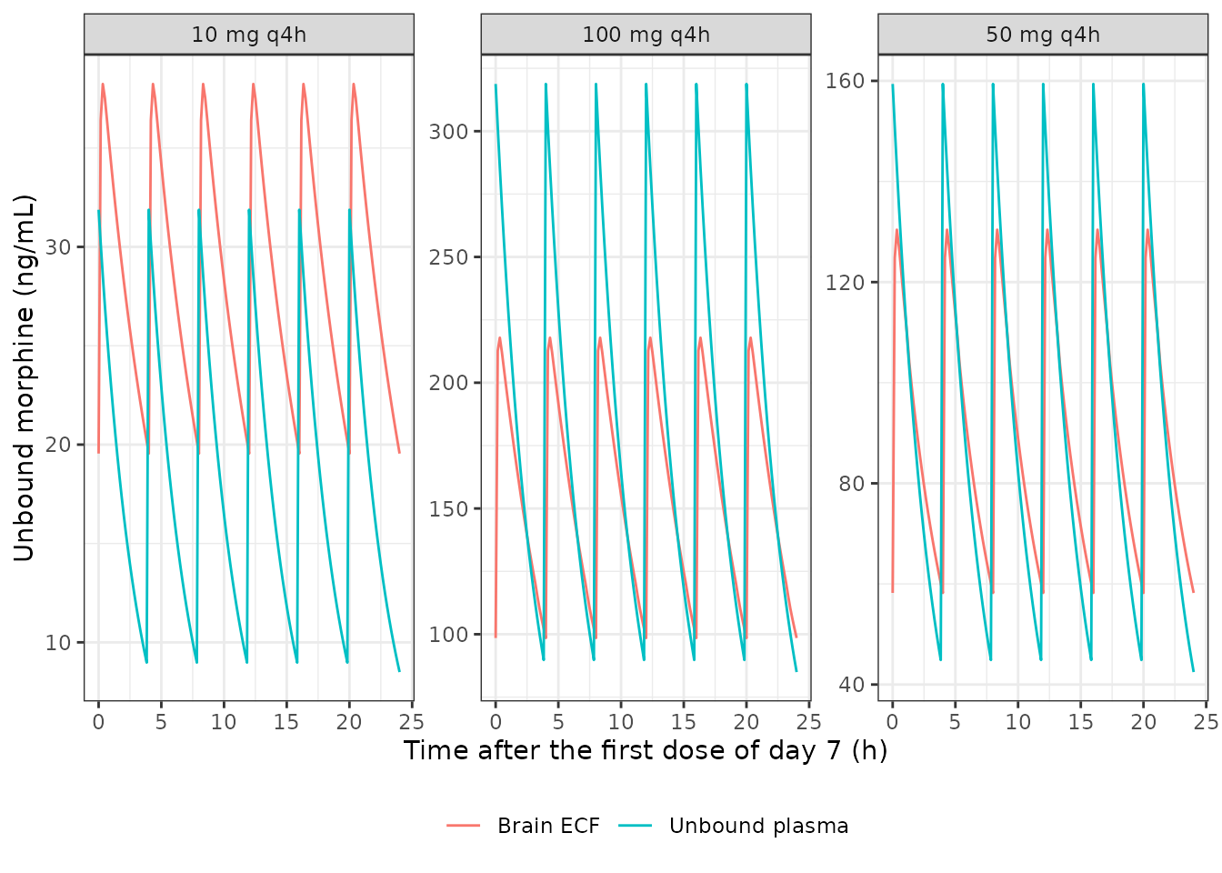
Typical-subject unbound plasma and brain-ECF morphine over day 7 for the three regimens, without inhibitor.
Figure 2: inhibitor effect across the virtual population
Replicates Figure 2 of Gulave 2025 for a subset of inhibitors spanning the range of the printed DDI column. Each subject keeps the same plasma PK in every arm, so the ratio isolates the inhibitor. The paper used 2000 subjects and reported up to the 99.9th percentile; with 200 subjects per arm the upper percentiles shown are the 95th, 99th and the maximum.
rxode2::rxSetSeed(20250107)
set.seed(20250107)
n_sub <- 200
etas <- tibble(sub = seq_len(n_sub),
  etalcl = rnorm(n_sub, 0, sqrt(0.222)),
  etalvc = rnorm(n_sub, 0, sqrt(0.747)))
fig2_inh <- c("verapamil", "chlorpromazine", "quinidine", "tariquidar",
  "amiodarone", "fluvoxamine", "loratadine")
fig2_arms <- tibble(inhibitor = c("none", fig2_inh)) |>
  left_join(select(inhibitors, inhibitor, ddi_printed), by = "inhibitor") |>
  mutate(INH_PGP_RATIO = coalesce(ddi_printed, 0), arm = row_number())
pop_pars <- expand_grid(arm = fig2_arms$arm, sub = etas$sub) |>
  left_join(etas, by = "sub") |>
  left_join(select(fig2_arms, arm, INH_PGP_RATIO), by = "arm") |>
  mutate(id = row_number())
sim2 <- suppressWarnings(rxSolve(mod_typ, regimen_events(10, ids = pop_pars$id),
  params = select(pop_pars, id, etalcl, etalvc, INH_PGP_RATIO),
  returnType = "data.frame", cores = 1L))
auc2 <- sim2 |>
  group_by(id) |>
  summarise(auc = trap_auc(time, Cbrain_ecf), .groups = "drop") |>
  left_join(select(pop_pars, id, arm, sub), by = "id") |>
  left_join(select(fig2_arms, arm, inhibitor), by = "arm")
ratio2 <- auc2 |>
  filter(inhibitor != "none") |>
  left_join(auc2 |> filter(inhibitor == "none") |> select(sub, auc_ctrl = auc), by = "sub") |>
  mutate(ratio = auc / auc_ctrl)
pct2 <- ratio2 |>
  group_by(inhibitor) |>
  summarise(p50 = median(ratio), p95 = quantile(ratio, 0.95),
    p99 = quantile(ratio, 0.99), max = max(ratio), .groups = "drop") |>
  arrange(desc(p99))
pct2 |>
  rename(Inhibitor = inhibitor, "Median" = p50, "95th pct" = p95,
    "99th pct" = p99, "Maximum" = max) |>
knitr::kable(digits = 4, caption = "AUC_ECF DDI ratio (inhibited / control), morphine 10 mg q4h, 200 subjects.")| Inhibitor | Median | 95th pct | 99th pct | Maximum |
|---|---|---|---|---|
| verapamil | 1.0085 | 1.0088 | 1.0388 | 1.0500 |
| chlorpromazine | 1.0085 | 1.0088 | 1.0388 | 1.0500 |
| quinidine | 1.0085 | 1.0088 | 1.0386 | 1.0498 |
| tariquidar | 1.0081 | 1.0083 | 1.0366 | 1.0471 |
| amiodarone | 1.0076 | 1.0078 | 1.0342 | 1.0440 |
| fluvoxamine | 1.0046 | 1.0048 | 1.0205 | 1.0263 |
| loratadine | 1.0000 | 1.0000 | 1.0000 | 1.0000 |
stopifnot(
  # Most of the population sees no effect (Figure 2: 95th percentile ~1.00).
  all(pct2$p50 < 1.01),
  # Robust envelope: the paper's maximum effect at the 99.9th percentile is
  # about 4%; allow headroom for the smaller cohort.
  all(pct2$p95 < 1.05)
)
ratio2 |>
  mutate(inhibitor = factor(inhibitor, levels = rev(pct2$inhibitor))) |>
  ggplot(aes(ratio, inhibitor)) +
  geom_boxplot(outlier.size = 0.6) +
  geom_vline(xintercept = 1, linetype = 2) +
  labs(x = "AUC_ECF DDI ratio (inhibited / control)", y = NULL) +
  theme_bw()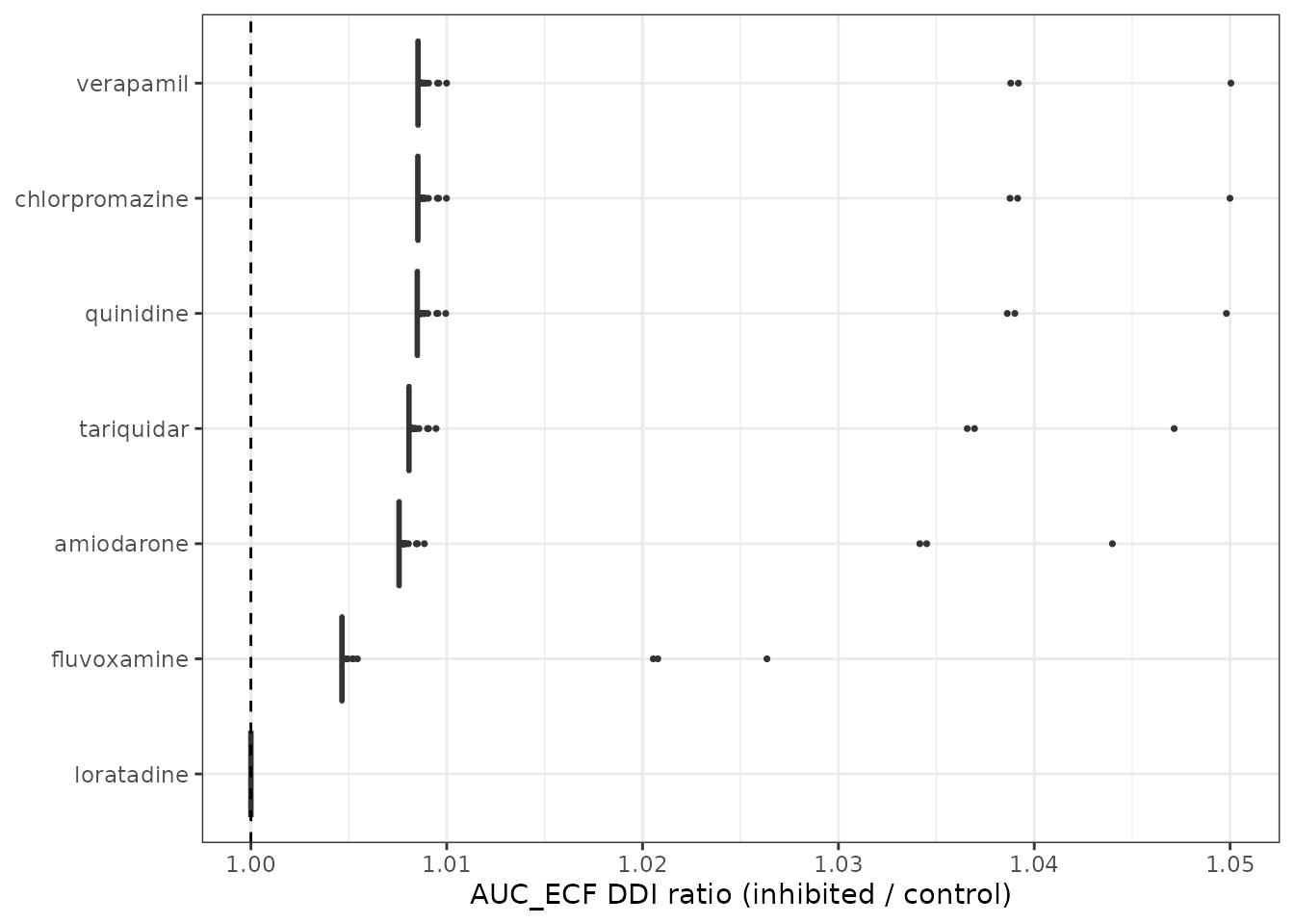
Replicates Figure 2 of Gulave 2025: distribution of the AUC_ECF DDI ratio across the virtual population (10 mg q4h).
Figure 3: sensitivity to the inhibitor parameters
Replicates Figure 3 of Gulave 2025 for the typical subject. Because
the inhibitor enters only through fu,p * [I] / Ki,
multiplying fu,p or the inhibitor concentration by a factor
f, or dividing Ki by f, multiplies the ratio
by f. The result is expressed relative to the unperturbed
inhibited condition, as in the figure.
fig3_inh <- c("loratadine", "tariquidar", "verapamil")
perturb <- tibble(
  parameter = rep(c("Fraction unbound inhibitor", "Inhibitor concentration", "Inhibitory constant"),
    c(3, 5, 5)),
  factor = c(0.1, 1, 10, 0.1, 1, 10, 100, 1000, 0.1, 1, 10, 100, 1000)
) |>
  mutate(ratio_multiplier = ifelse(parameter == "Inhibitory constant", 1 / factor, factor))
# rxSolve aligns a params data.frame to the event table by ROW ORDER, not by
# matching the id column, so the ev_g3 ids must appear in the same order as the
# params rows. ev_g3 is built dose by dose, so grid3 is arranged by dose first
# and its id assigned afterwards; both are then in ascending-id order.
grid3 <- expand_grid(dose_mg = c(10, 50, 100), inhibitor = fig3_inh,
  ratio_multiplier = unique(perturb$ratio_multiplier)) |>
  arrange(dose_mg) |>
  left_join(select(inhibitors, inhibitor, ddi_printed), by = "inhibitor") |>
  mutate(base = ifelse(inhibitor == "loratadine", loratadine_ddi, ddi_printed),
    INH_PGP_RATIO = base * ratio_multiplier, id = row_number())
ev_g3 <- bind_rows(lapply(c(10, 50, 100), function(mg) {
  ids <- grid3$id[grid3$dose_mg == mg]
  as.data.frame(regimen_events(mg, ids = ids))
}))
sim_g3 <- rxSolve(mod_typ, ev_g3, params = select(grid3, id, INH_PGP_RATIO),
  returnType = "data.frame", cores = 1L)
#> ℹ omega/sigma items treated as zero: 'etalcl', 'etalvc'
#> Warning: multi-subject simulation without without 'omega'
auc_g3 <- sim_g3 |>
  group_by(id) |>
  summarise(auc = trap_auc(time, Cbrain_ecf), .groups = "drop") |>
  left_join(grid3, by = "id")
fig3 <- perturb |>
  left_join(auc_g3, by = "ratio_multiplier", relationship = "many-to-many") |>
  group_by(inhibitor, dose_mg) |>
  mutate(change = auc / auc[ratio_multiplier == 1][1]) |>
  ungroup()
ggplot(fig3, aes(factor(factor), factor(dose_mg), fill = change)) +
  geom_tile(colour = "white") +
  facet_grid(inhibitor ~ parameter, scales = "free_x") +
  scale_fill_gradient2(low = "#2b2d6e", mid = "white", high = "#e8432d",
    midpoint = 1, limits = c(0.85, 1.12)) +
  labs(x = "Perturbation factor", y = "Morphine dose (mg q4h)", fill = "Change\nnew/original") +
  theme_bw()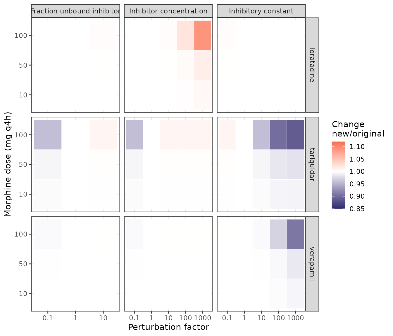
Replicates Figure 3 of Gulave 2025: brain-ECF AUC relative to the unperturbed inhibited condition.
Values read off the published heat map compared with the model (100 mg q4h):
fig3_ref <- tibble::tribble(
  ~inhibitor, ~parameter, ~factor, ~published,
  "tariquidar", "Fraction unbound inhibitor", 0.1, 0.91,
  "tariquidar", "Inhibitor concentration", 0.1, 0.91,
  "tariquidar", "Inhibitory constant", 100, 0.88,
  "tariquidar", "Inhibitory constant", 1000, 0.86,
  "verapamil", "Inhibitory constant", 1000, 0.89,
  "loratadine", "Inhibitor concentration", 1000, 1.08
)
fig3_cmp <- fig3_ref |>
  left_join(fig3 |> filter(dose_mg == 100) |> select(inhibitor, parameter, factor, change),
    by = c("inhibitor", "parameter", "factor"))
fig3_cmp |>
  rename(Inhibitor = inhibitor, Parameter = parameter, "Perturbation" = factor,
    "Figure 3 (read from colour scale)" = published, "Model" = change) |>
knitr::kable(digits = 3, caption = "Figure 3 at 100 mg q4h: digitised colour values versus the model.")| Inhibitor | Parameter | Perturbation | Figure 3 (read from colour scale) | Model |
|---|---|---|---|---|
| tariquidar | Fraction unbound inhibitor | 1e-01 | 0.91 | 0.958 |
| tariquidar | Inhibitor concentration | 1e-01 | 0.91 | 0.958 |
| tariquidar | Inhibitory constant | 1e+02 | 0.88 | 0.901 |
| tariquidar | Inhibitory constant | 1e+03 | 0.86 | 0.888 |
| verapamil | Inhibitory constant | 1e+03 | 0.89 | 0.908 |
| loratadine | Inhibitor concentration | 1e+03 | 1.08 | 1.090 |
stopifnot(
  # At 10 mg (Kp,uu,BBB > 1) the published panel is uniformly white.
  all(abs(fig3$change[fig3$dose_mg == 10] - 1) < 0.02),
  # Same direction as the figure in every compared cell, within the
  # resolution of a colour-scale read-off.
  all(sign(fig3_cmp$change - 1) == sign(fig3_cmp$published - 1)),
  all(abs(fig3_cmp$change - fig3_cmp$published) < 0.06)
)
Figure 4: sensitivity to the translation factor fAF_BBB
Replicates Figure 4 of Gulave 2025: 10 mg q4h, tariquidar at 1, 10 and 100 times its clinical concentration, for fAF_BBB of 0.1, 0.22, 0.3 and 1. The AUC is relative to fAF_BBB = 0.218 with the same tariquidar concentration.
fig4 <- expand_grid(faf = c(0.21815, 0.1, 0.3, 1), fold = c(1, 10, 100)) |>
  rowwise() |>
  mutate(auc = auc_ecf_typical(10, 16.8 * fold, extra = c(faf_bbb = faf))) |>
  ungroup() |>
  group_by(fold) |>
  mutate(change = auc / auc[faf == 0.21815]) |>
  ungroup()
#> ℹ omega/sigma items treated as zero: 'etalcl', 'etalvc'
#> ℹ omega/sigma items treated as zero: 'etalcl', 'etalvc'
#> ℹ omega/sigma items treated as zero: 'etalcl', 'etalvc'
#> ℹ omega/sigma items treated as zero: 'etalcl', 'etalvc'
#> ℹ omega/sigma items treated as zero: 'etalcl', 'etalvc'
#> ℹ omega/sigma items treated as zero: 'etalcl', 'etalvc'
#> ℹ omega/sigma items treated as zero: 'etalcl', 'etalvc'
#> ℹ omega/sigma items treated as zero: 'etalcl', 'etalvc'
#> ℹ omega/sigma items treated as zero: 'etalcl', 'etalvc'
#> ℹ omega/sigma items treated as zero: 'etalcl', 'etalvc'
#> ℹ omega/sigma items treated as zero: 'etalcl', 'etalvc'
#> ℹ omega/sigma items treated as zero: 'etalcl', 'etalvc'
fig4_ref <- tibble(faf = c(0.1, 0.3, 1), published = c(0.83, 1.12, 2.15))
fig4_cmp <- fig4 |>
  filter(fold == 1, faf != 0.21815) |>
  select(faf, change) |>
  left_join(fig4_ref, by = "faf")
fig4_cmp |>
  rename("fAF_BBB" = faf, "Model" = change, "Figure 4 (read from bars)" = published) |>
knitr::kable(digits = 3, caption = "Brain-ECF AUC fold change versus fAF_BBB = 0.218 (tariquidar 1x).")| fAF_BBB | Model | Figure 4 (read from bars) |
|---|---|---|
| 0.1 | 0.788 | 0.83 |
| 0.3 | 1.147 | 1.12 |
| 1.0 | 2.400 | 2.15 |
stopifnot(
  # Tariquidar concentration does not change the fAF response (Figure 4).
  max(abs(fig4$change[fig4$fold == 100] - fig4$change[fig4$fold == 1])) < 0.02,
  all(abs(fig4_cmp$change / fig4_cmp$published - 1) < 0.15)
)
fig4 |>
  mutate(faf = factor(signif(faf, 2), levels = c("0.22", "0.1", "0.3", "1"))) |>
  ggplot(aes(faf, change, fill = factor(fold))) +
  geom_col(position = "dodge") +
  geom_hline(yintercept = 1, linetype = 2) +
  labs(x = "Interspecies conversion factor (fAF_BBB)", y = "AUC fold change",
    fill = "Tariquidar\nconcentration fold") +
  theme_bw()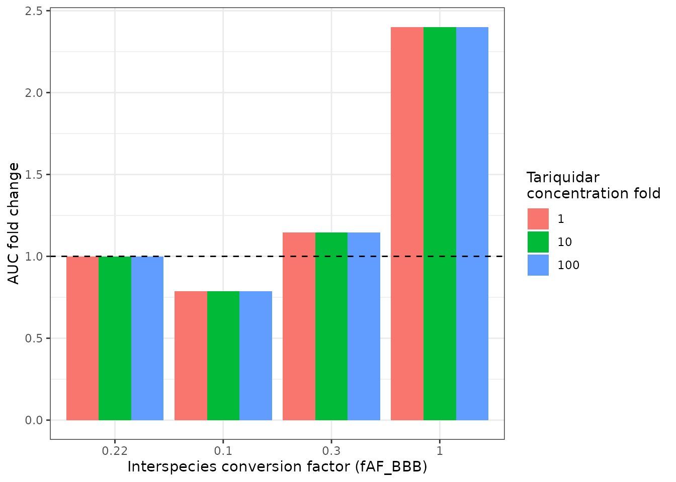
Replicates Figure 4 of Gulave 2025.
Assumptions and deviations
Assumptions
-
Kp,uu,BBB is evaluated at the instantaneous unbound plasma
concentration. Table 1 writes the function in terms of
Css,u,plasma, the variable it was fitted against in rat steady-state simulations. Applying it to the time-varying concentration is what makes brain-ECF fluctuation dose-dependent, which Gulave 2023 reports, and it reproduces the paper’s regimen classification and Figures 3-4. - How fAF_BBB enters. Neither the paper nor Gulave 2023 prints the formula. The model multiplies the back-calculated BBB asymmetry factor (influx when Kp,uu,BBB >= 1, efflux when < 1) by fAF_BBB, the method of Yamamoto et al. 2018 (human AF = rat AF x expression ratio), and the only reading consistent with the published sensitivity directions: a larger fAF_BBB raises brain-ECF exposure at low doses (influx scaled) and lowers it at high doses (efflux scaled; Gulave 2023 Section 3.4), and Figure 4’s 10 mg bars rise with fAF_BBB. The factor fixed at 1 is not scaled. The closed forms are evaluated with human physiology.
- Where the DDI enters. The asymmetry factors are computed without the inhibitor (Supplementary Eqs. 3-4 as printed) and the inhibitor then divides the transcellular efflux term (Eq. 3). Back-solving the influx factor with the inhibited efflux factor instead changes the 10 mg results by under 0.5% and the 100 mg results not at all.
- Kp,uu at the blood-CSF barrier is not reported for morphine and is set equal to Kp,uu,BBB, as the LeiCNS-PK3.0 authors’ default. The fAF_BBB scaling and the DDI are applied at the BBB only. CSF compartments are downstream of brain ECF, so this does not affect the brain-ECF endpoint.
- Morphine is given as IV bolus doses. The paper says “intravenous dosing” without an infusion duration.
- Plasma is a forcing function, as in all LeiCNS-PK3.0 models: CNS uptake does not deplete plasma.
- The human brain-cell-membrane (phospholipid) volume is 5% of the 1250 mL total brain volume, the LeiCNS-PK3.0 definition. The BCSFB width and the microvasculature pH are merged cells in Saleh 2021 Supplementary Table 2 (0.5 um and 7.4).
Source issues, carried through as published
-
The printed DDI column of Supplementary Table 1 is 1000-fold
larger than fu,p x Css / Ki in consistent units. Css is in
ng/mL and Ki in uM, so the dimensionless term needs Css converted to uM
through the inhibitor molecular weight. For verapamil (454.6 g/mol): 0.1
x 498 / 454.6 = 0.110 uM, divided by Ki = 0.3 uM gives 0.365; the table
prints 365.1. Tariquidar (646.7 g/mol) gives 0.0168 against a printed
16.8. Every row checked (amiodarone, amisulpride, chlorpromazine,
diltiazem, haloperidol, quinidine and others) matches Css converted to
nmol/L divided by Ki in umol/L, i.e. a missing nM-to-uM step. The
published simulations used the printed values: with them the model
reproduces Figure 3, including the loratadine increase at 1000-fold
concentration and the verapamil effect appearing only at a 1000-fold Ki,
and the text’s statement that verapamil’s Ki stays below fu,p x C even
after a 100-fold increase holds only on the printed scale. This vignette
therefore uses the printed values to replicate the figures.
INH_PGP_RATIOitself is defined as the dimensionless ratio; a user computing it in consistent units will get inhibitor effects 1000 times smaller than the paper’s, i.e. none. -
The Kp,uu,BBB function differs from the one printed in
Gulave 2023 (
5.4902 x Css,u,plasma^-0.552), although the paper cites that work for it. The model uses this paper’s Table 1 function, which reproduces the stated regimen classification (10 mg above 1, 50 mg around 1, 100 mg below 1); the 2023 power function would put the crossover near 22 ng/mL instead of 109 ng/mL. - Supplementary equations 3-4 state the condition “Kp,uu,BBB < 1” twice. The first should read “> 1” (influx factor back-calculated); the model uses the selection rule of Saleh 2021 and Gulave 2023.
- The Results text says fu,p was perturbed by 0.1 and 10; the figure legend agrees. The 10-fold fu,p perturbation exceeds 1 for several inhibitors; it is reproduced as a ratio multiplier.
Deviations
- 200 virtual subjects per arm instead of 2000, so Figure 2’s 99.9th percentile is not estimable; the replication reports the median, 95th, 99th percentile and maximum, for seven of the 34 inhibitors.
- Figure 3 and Figure 4 are replicated for the typical subject; the paper does not say whether its sensitivity runs used the typical subject or a population summary. Model and figure agree in direction for every compared cell and within 0.06 on the colour scale for Figure 3; for Figure 4 the model gives 0.79 / 1.15 / 2.40 against about 0.83 / 1.12 / 2.15 read from the bars. No parameter was adjusted to close these gaps.
- The paper reports no absolute NCA values, so no published-versus-simulated NCA table is possible; the PKNCA block above reproduces the paper’s two relative metrics.
- The morphine metabolites M3G and M6G, part of Gulave 2023 and of the Oosten 2017 plasma model, are not part of this paper’s analysis and are not included.