Tenecteplase (Tang 2023)
Source:vignettes/articles/Tang_2023_tenecteplase.Rmd
Tang_2023_tenecteplase.RmdModel and source
- Citation: Tang F, Langenhorst J, Dang S, Kassir N, Owen R, Purdon B, Magnusson MO, Deng R (2023). Population Pharmacokinetics of Tenecteplase in Patients With Acute Myocardial Infarction and Application to Patients With Acute Ischemic Stroke. The Journal of Clinical Pharmacology 63(2):197-209. doi:10.1002/jcph.2164.
- Description: Two-compartment linear population PK model for intravenous bolus tenecteplase in adults with acute myocardial infarction (Tang 2023; phase II TIMI 10B, 785 plasma concentrations from 103 patients). Clearance is the sum of a renal-function-independent intercept and an additive linear effect of Cockcroft-Gault creatinine clearance normalized to 70 kg body weight (CRCL-NM), centered on the cohort median 82.6 mL/min/70 kg; allometric body-weight scaling is fixed at 0.75 on CL and Q and 1 on Vc and Vp with a 70 kg reference. Because the sandwich ELISA cannot distinguish tenecteplase from endogenous tissue plasminogen activator, the predicted observation is the sum of the model-predicted tenecteplase concentration and a per-subject background signal (bl_tpa, typical 18.6 ng/mL). Inter-individual variability on Vc is perfectly correlated with that on CL and is constructed as vc_eta_scale * etalcl; the log-additive residual error itself carries inter-individual variability on its magnitude. The authors caution that the statistically selected renal contribution to clearance is biologically implausible for a 65 kDa protein cleared mainly by hepatic metabolism, and that it may reflect collinearity between CRCL-NM, age and serum creatinine in the stepwise covariate search.
- Article: https://doi.org/10.1002/jcph.2164
- Supplement (Tables S1-S5, Figures S1-S2): open-access supporting information distributed with the article via PubMed Central (PMC10099546).
Population
The model was developed from the phase II TIMI 10B study in adults with acute myocardial infarction: 785 plasma concentrations from 103 tenecteplase-treated patients. Patients were randomized to a single intravenous bolus of 30 mg (n = 52), 40 mg (n = 31) or 50 mg (n = 20); the 50 mg arm was suspended on 22 August 1996 and replaced by 40 mg after three intracranial hemorrhages among 78 patients dosed at 50 mg. All patients received 150-325 mg of aspirin daily plus heparin.
Baseline characteristics (Table S1, all doses pooled): body weight 84.1 +/- 20.0 kg, age 56.4 +/- 11.4 years, Cockcroft-Gault creatinine clearance normalized to 70 kg (CRCL-NM) 83.3 +/- 25.5 mL/min/70 kg, serum creatinine 1.08 +/- 0.956 mg/dL, AST 38.9 +/- 42.1 U/L, ALT 53.7 +/- 33.5 U/L. 75 of 103 patients (72.8%) were male. Race was 69.9% White, 13.6% Black, 13.6% Hispanic, 1.9% other, 1.0% Asian. The reference patient used throughout the paper’s own simulations is the cohort median: 81.8 kg and 82.6 mL/min/70 kg.
PK samples were drawn at baseline and 2, 30, 60, 90, 120, 180 and 360 minutes after the start of administration; all were above the 8 ng/mL lower limit of quantification.
The same information is available programmatically via
readModelDb("Tang_2023_tenecteplase")()$population.
Model structure
Tenecteplase PK is a two-compartment linear model with intravenous bolus dosing. Body weight scales all disposition parameters allometrically on a 70 kg reference, with exponents fixed at 0.750 (CL, Q) and 1.00 (Vc, Vp); the paper constrains the exponent to be shared between CL and Q and between Vc and Vp. Clearance additionally carries an additive linear effect of CRCL-NM centered on the cohort median (Eq. 9):
Equation 8 shows the identical model written as the sum of a renal
and a nonrenal clearance, which is where the interpretation of
e_crcl_cl = 0.322 as “the renal CL of tenecteplase relative
to that of creatinine” comes from. The implied nonrenal clearance is
91.3 - 0.322 * 82.6 = 64.7 mL/min, so clearance stays
positive across the whole physiological CRCL-NM range.
Because the sandwich ELISA cannot distinguish tenecteplase from
endogenous tissue plasminogen activator, the predicted observation is
the sum of the model-predicted tenecteplase concentration and a
per-subject background signal (Eq. 2): yhat = C + BS. The
residual error is log-additive (Eq. 3) and, unusually, carries its own
inter-individual variability on the residual magnitude, which the
authors introduced to reduce the leverage of outliers without excluding
observations.
A caution the authors state explicitly. Tenecteplase is a 65 kDa protein cleared mainly by hepatic metabolism, so a 29% renal contribution to clearance is not biologically expected. The Discussion warns that “given the biological unlikelihood of a renal contribution to CL, statistical significance of CRCL-NM needs to be interpreted with caution”, and notes that CRCL-NM, age and serum creatinine were strongly collinear (Figure S2). An alternative covariate analysis that removed CRCL-NM and CREA from the structural set instead selected age and race on CL (run 50, Table S4) with a worse OFV. The packaged model reproduces the paper’s final model (run 34); the alternative model is not encoded.
Source trace
| Equation / parameter | Value | Source location |
|---|---|---|
| Two-compartment linear structure | n/a | Abstract; Results “Model Development” (run 17 base model) |
Exponential IIV theta_pi = theta_p * exp(eta_pi)
|
n/a | Equation 1 |
Observation yhat = C + BS
|
n/a | Equation 2 |
Log-additive residual with IIV
log y = log yhat + eps * exp(eta)
|
n/a | Equation 3 |
Allometric form (WT/70)^theta
|
n/a | Equation 6 |
| Final CL covariate model | n/a | Equation 9 (run 34) |
lcl (CL at WT 70 kg, CRCL-NM 82.6) |
91.3 mL/min | Table 1 “CL, mL/min” (RSE 2.52%); Table S4 final-model column |
lvc (Vc at WT 70 kg) |
3610 mL | Table 1 “Vc, mL” (RSE 2.94%) |
lq (Q at WT 70 kg) |
10.0 mL/min | Table 1 “Q, mL/min” (RSE 5.89%) |
lvp (Vp at WT 70 kg) |
914 mL | Table 1 “Vp, mL” (RSE 5.70%) |
e_wt_cl_q (fixed) |
0.750 | Table 1 “Exponent for WT on CL and Q”, no RSE; Results run 13 |
e_wt_vc_vp (fixed) |
1.00 | Table 1 “Exponent for WT on volume”, no RSE; Results run 13 |
e_crcl_cl |
0.322 | Table 1 “CRCL-NM effect on CL” (RSE 10.6%); Eq. 9 |
lbl_tpa (background signal BS) |
18.6 ng/mL | Table 1 “BS, ng/mL” (RSE 5.48%); Eq. 2 |
vc_eta_scale |
0.913 | Table 1 “IIV CL - IIV Vc scaler” (RSE 5.87%); Results run 7 |
etalcl |
SD 0.199 | Table 1 “IIV CL, CV” (RSE 11.0%, shrinkage 12.0%) |
etalbl_tpa |
SD 0.285 | Table 1 “IIV BS, CV” (RSE 18.5%, shrinkage 25.5%) |
etaexpSd |
SD 0.789 | Table 1 “IIV RUV, CV” (RSE 10.7%, shrinkage 0%) |
expSd |
0.311 | Table 1 “LogAdd RUV tenecteplase, CV” (RSE 7.74%) |
| Reference patient (WT, CRCL-NM) | 81.8 kg, 82.6 mL/min/70 kg | Results “Evaluation of Covariate Effect by Simulation” |
Note on the variance scale
Table 1 heads its variability column “CV”, but the values are
omega standard deviations on the exponential-IIV scale
of Eq. 1, not variances and not sqrt(exp(omega^2) - 1)
coefficients of variation. Two independent signals fix this:
- The Table S3 and Table S4 captions state “The RSE for IIV and RUV parameters is reported on the approximate SD scale.”
- The final row of the same column is the log-additive residual error, whose sigma on the log scale is its approximate CV. A column that mixed a log-scale sigma with lognormal CVs computed by back-transformation would not be internally consistent.
Methods Eq. 1 also defines eta_pi as “a normally
distributed random variable with mean 0 and standard deviation (SD)
omega_p”. The model file therefore records
omega^2 = SD^2.
mod <- readModelDb("Tang_2023_tenecteplase")
ui  <- rxode2::rxode(mod)
#> ℹ parameter labels from comments will be replaced by 'label()'

# Reference patient used by the paper's own simulations.
WT_REF   <- 81.8   # kg,             cohort median (Results)
CRCL_REF <- 82.6   # mL/min/70 kg,   cohort median (Eq. 9 centering constant)
Deterministic checks against published values
These use rxode2::zeroRe() so they are typical-value
predictions with no between-subject variability, and are therefore
exactly reproducible on any machine. Each compares the model against a
number the paper prints.
# Dense grid: fine through the distribution phase (alpha t1/2 ~ 21 min), then
# out to 1440 min (~19 terminal half-lives) so the AUC extrapolation is
# negligible without pushing the solve into numerical noise.
TGRID <- sort(unique(c(
  seq(0, 30, by = 0.25), seq(30, 120, by = 1),
  seq(120, 360, by = 2), seq(360, 1440, by = 10)
)))

mod_typ <- rxode2::zeroRe(mod)
#> ℹ parameter labels from comments will be replaced by 'label()'
#> Warning: No sigma parameters in the model

# Solve one typical-value profile per row of `spec` (id, amt, WT, CRCL, label).
solve_typical <- function(spec) {
  dose <- spec |>
    dplyr::mutate(time = 0, evid = 1L, cmt = "central") |>
    dplyr::select(id, time, amt, evid, cmt, WT, CRCL, label)
  obs <- spec |>
    dplyr::select(id, WT, CRCL, label) |>
    tidyr::crossing(time = TGRID) |>
    dplyr::mutate(amt = NA_real_, evid = 0L, cmt = "central")
  ev <- dplyr::bind_rows(dose, obs) |>
    dplyr::arrange(id, time, dplyr::desc(evid))
  rxode2::rxSolve(mod_typ, ev, keep = c("WT", "CRCL", "label"),
                  returnType = "data.frame")
}

# Tenecteplase-only concentration. `Cc` is what the assay reports, i.e.
# tenecteplase PLUS the endogenous t-PA background (Eq. 2), but the paper's
# AUC is dose/CL, which is the tenecteplase AUC. Integrating `Cc` unchanged
# would add bl_tpa * T to every AUC (a ~28% inflation over this window), so
# the background is removed before any NCA or integration.
tnk_conc <- function(sim) sim$Cc - sim$bl_tpa

# Trapezoidal AUC of the tenecteplase concentration, ug*min/mL.
auc_trapz <- function(d) {
  d <- d[order(d$time), ]
  cc <- tnk_conc(d)
  sum(diff(d$time) * (utils::head(cc, -1) + utils::tail(cc, -1)) / 2) / 1000
}
Reference-patient clearance and the renal fraction
ref <- data.frame(id = 1L, amt = 0.25 * WT_REF, WT = WT_REF,
                  CRCL = CRCL_REF, label = "reference")
sim_ref <- solve_typical(ref)
#> ℹ omega/sigma items treated as zero: 'etalcl', 'etalbl_tpa', 'etaexpSd'

cl_model <- unique(round(sim_ref$cl, 6))
stopifnot(length(cl_model) == 1L)

# Renal fraction of total CL at the median covariate values, from the model's
# own coefficients: e_crcl_cl * CRCL_REF / CL_pop.
theta_crcl <- ui$theta[["e_crcl_cl"]]
cl_pop     <- exp(ui$theta[["lcl"]])
renal_frac <- 100 * theta_crcl * CRCL_REF / cl_pop

cat(sprintf("Reference-patient CL : %.1f mL/min   (paper Discussion: 103)\n", cl_model))
#> Reference-patient CL : 102.6 mL/min   (paper Discussion: 103)
cat(sprintf("Renal fraction of CL : %.1f%%          (paper Results: 29.2%%)\n", renal_frac))
#> Renal fraction of CL : 29.1%          (paper Results: 29.2%)

# Deterministic quantities -- safe to assert tightly.
stopifnot(
  abs(cl_model - 103) / 103 < 0.01,
  abs(renal_frac - 29.2) < 0.5
)
Published AUC anchors
The paper reports simulated median AUC for a reference patient at
four dose levels, derived as dose/CL (Methods: “AUC from
the time of dosing to infinity was used as derived from dose/CL”).
Reproducing these exercises the covariate model, the allometric scaling,
the centering constant and the mg-to-ng unit conversion in one number
each. The AUC below is obtained by integrating the solved ODE
profile, not from the model’s cl variable, so an
error in the compartment structure would show up here.
anchors <- tibble::tribble(
  ~label,        ~amt,             ~published_auc,
  "0.1 mg/kg",   0.1 * WT_REF,      79.7,   # Results: "0.1 mg/kg (79.7 ug*min/mL)"
  "0.25 mg/kg",  0.25 * WT_REF,     NA,     # 90% PI 145-256; checked separately
  "0.5 mg/kg",   0.5 * WT_REF,     398,     # Results: "0.5 mg/kg (398 ug*min/mL)"
  "50 mg",      50,                487      # Results: "50 mg (487 ug*min/mL)"
) |>
  dplyr::mutate(id = dplyr::row_number(), WT = WT_REF, CRCL = CRCL_REF)

sim_anchor <- solve_typical(anchors)
#> ℹ omega/sigma items treated as zero: 'etalcl', 'etalbl_tpa', 'etaexpSd'
#> Warning: multi-subject simulation without without 'omega'
stopifnot(all(tnk_conc(sim_anchor) >= 0))   # no solver noise in the tail

auc_tab <- sim_anchor |>
  dplyr::group_by(label) |>
  dplyr::group_modify(~ tibble::tibble(auc_model = auc_trapz(.x))) |>
  dplyr::ungroup() |>
  dplyr::left_join(dplyr::select(anchors, label, published_auc), by = "label") |>
  dplyr::mutate(pct_diff = 100 * (auc_model - published_auc) / published_auc)

auc_tab |>
  dplyr::rename(
    "Dose level"                = label,
    "Model AUC (ug*min/mL)"     = auc_model,
    "Published AUC (ug*min/mL)" = published_auc,
    "Difference (%)"            = pct_diff
  ) |>
  knitr::kable(digits = c(0, 1, 1, 2),
caption = "AUC from the integrated ODE solve vs the published simulated median AUC for the reference patient (81.8 kg, CRCL-NM 82.6 mL/min/70 kg). Replicates the dose-level values quoted in Results, 'Evaluation of Covariate Effect by Simulation'.")| Dose level | Model AUC (ug*min/mL) | Published AUC (ug*min/mL) | Difference (%) |
|---|---|---|---|
| 0.1 mg/kg | 79.7 | 79.7 | 0.02 |
| 0.25 mg/kg | 199.3 | NA | NA |
| 0.5 mg/kg | 398.6 | 398.0 | 0.15 |
| 50 mg | 487.3 | 487.0 | 0.06 |
# The 0.25 mg/kg row has no published point estimate, only a 90% prediction
# interval of 145-256 ug*min/mL reflecting parameter uncertainty.
auc_025 <- auc_tab$auc_model[auc_tab$label == "0.25 mg/kg"]
stopifnot(length(auc_025) == 1L)
cat(sprintf("0.25 mg/kg model AUC: %.1f ug*min/mL (published 90%% PI 145-256)\n", auc_025))
#> 0.25 mg/kg model AUC: 199.3 ug*min/mL (published 90% PI 145-256)

# Deterministic: tolerance is set by the paper's 3-significant-figure rounding,
# not by a single run. Realised differences are all under 0.2%.
stopifnot(
  max(abs(auc_tab$pct_diff), na.rm = TRUE) < 1,
  auc_025 > 145, auc_025 < 256
)
Replicate Figure 5: isolated covariate effects on AUC
Figure 5 presents forest plots of simulated AUC across renal-function
strata and weight groups relative to the reference patient, with an
80%-125% band. The paper’s conclusion is that “simulated tenecteplase
exposure mostly did not surpass the 80%-125% limits”, in contrast to the
dose changes checked above, which move exposure far outside it. Both
panels below dose 0.25 mg/kg, so the weight panel carries the
WT^0.25 net effect of a weight-proportional dose against
WT^0.75 clearance scaling.
renal_strata <- tibble::tribble(
  ~label,                       ~CRCL,
  "Moderate-severe (<60)",       45,
  "Mild (60-90)",                75,
  "Normal (90-120)",            105,
  "Supranormal (>=120)",        135
) |>
  dplyr::mutate(WT = WT_REF, amt = 0.25 * WT_REF, panel = "CRCL-NM (mL/min/70 kg)")

# Weight groups spanning the cohort (84.1 +/- 20.0 kg, Table S1).
weight_groups <- tibble::tibble(
  WT = c(60, 72, 82, 95, 110)
) |>
  dplyr::mutate(label = paste0(WT, " kg"), CRCL = CRCL_REF,
                amt = 0.25 * WT, panel = "Body weight")

cov_spec <- dplyr::bind_rows(renal_strata, weight_groups) |>
  dplyr::mutate(id = dplyr::row_number())

sim_cov <- solve_typical(cov_spec)
#> ℹ omega/sigma items treated as zero: 'etalcl', 'etalbl_tpa', 'etaexpSd'
#> Warning: multi-subject simulation without without 'omega'

forest <- sim_cov |>
  dplyr::group_by(label) |>
  dplyr::group_modify(~ tibble::tibble(auc = auc_trapz(.x))) |>
  dplyr::ungroup() |>
  dplyr::left_join(dplyr::select(cov_spec, label, panel), by = "label") |>
  dplyr::mutate(ratio_pct = 100 * auc / auc_025,
                label = factor(label, levels = rev(cov_spec$label)))

ggplot(forest, aes(ratio_pct, label)) +
  annotate("rect", xmin = 80, xmax = 125, ymin = -Inf, ymax = Inf,
           alpha = 0.15, fill = "steelblue") +
  geom_vline(xintercept = 100, linetype = "dashed") +
  geom_point(size = 2.5) +
  facet_grid(panel ~ ., scales = "free_y", space = "free_y") +
  labs(x = "AUC relative to the reference patient (%)", y = NULL,
       title = "Figure 5 - isolated covariate effects on tenecteplase AUC",
       caption = "Replicates Figure 5 of Tang 2023. Shaded band is 80%-125%; reference is 81.8 kg, CRCL-NM 82.6, 0.25 mg/kg.")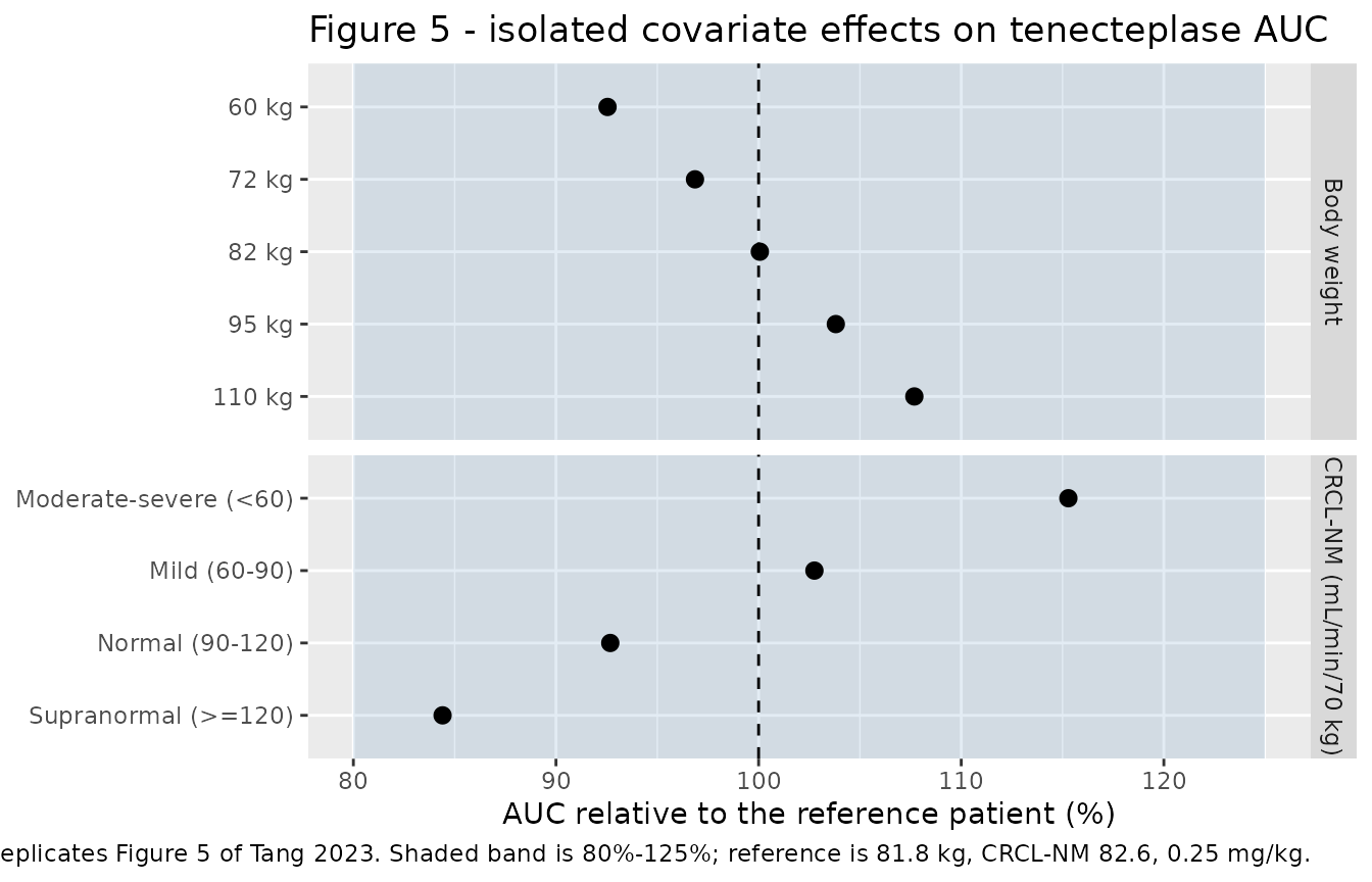
forest |>
  dplyr::select(panel, label, ratio_pct) |>
  dplyr::rename("Panel" = panel, "Group" = label,
                "AUC vs reference (%)" = ratio_pct) |>
knitr::kable(digits = 1, caption = "Typical-value AUC relative to the reference patient.")| Panel | Group | AUC vs reference (%) |
|---|---|---|
| Body weight | 110 kg | 107.7 |
| Body weight | 60 kg | 92.5 |
| Body weight | 72 kg | 96.9 |
| Body weight | 82 kg | 100.1 |
| Body weight | 95 kg | 103.8 |
| CRCL-NM (mL/min/70 kg) | Mild (60-90) | 102.8 |
| CRCL-NM (mL/min/70 kg) | Moderate-severe (<60) | 115.3 |
| CRCL-NM (mL/min/70 kg) | Normal (90-120) | 92.7 |
| CRCL-NM (mL/min/70 kg) | Supranormal (>=120) | 84.4 |
# The paper's published claim: covariate effects stay inside 80%-125%, whereas
# the 0.1 / 0.5 mg/kg dose changes sit far outside it. Deterministic values.
stopifnot(all(forest$ratio_pct > 80), all(forest$ratio_pct < 125))

# Contrast: the dose levels the paper calls "substantially outside" the band.
dose_ratio <- 100 * auc_tab$auc_model / auc_025
stopifnot(min(dose_ratio) < 60, max(dose_ratio) > 190)
Virtual cohort and Figure 1
# `set.seed()` seeds R's RNG for the covariate draws below. It does NOT seed
# rxode2's simulation RNG, and rxode2's streams are partitioned per solver
# thread, so the simulated etas differ between a 2-core CI runner and a
# 16-thread workstation. Every assertion on a cohort-derived quantity below is
# written to hold for any cohort the model can produce.
set.seed(20230201)
rxode2::rxSetSeed(20230201)

N_PER_ARM <- 200L   # cap is 200/arm

# Covariates drawn to match Table S1 (all doses pooled), truncated to keep
# weight and renal function physiological.
make_cohort <- function(n, dose_mg, arm, id_offset = 0L) {
  subj <- tibble::tibble(
    id   = id_offset + seq_len(n),
    WT   = pmin(pmax(stats::rnorm(n, 84.1, 20.0), 45), 150),
    CRCL = pmin(pmax(stats::rnorm(n, 83.3, 25.5), 20), 170),
    arm  = arm,
    doseMg = dose_mg
  )
  dose <- subj |>
    dplyr::mutate(time = 0, amt = dose_mg, evid = 1L, cmt = "central")
  obs <- subj |>
    tidyr::crossing(time = c(0, 2, 30, 60, 90, 120, 180, 360)) |>
    dplyr::mutate(amt = NA_real_, evid = 0L, cmt = "central")
  dplyr::bind_rows(dose, obs) |> dplyr::arrange(id, time, dplyr::desc(evid))
}

events <- dplyr::bind_rows(
  make_cohort(N_PER_ARM, 30, "30 mg", id_offset =    0L),
  make_cohort(N_PER_ARM, 40, "40 mg", id_offset = 1000L),
  make_cohort(N_PER_ARM, 50, "50 mg", id_offset = 2000L)
)
stopifnot(!anyDuplicated(unique(events[, c("id", "time", "evid")])))
sim <- rxode2::rxSolve(mod, events = events,
                       keep = c("WT", "CRCL", "arm", "doseMg"),
                       returnType = "data.frame")
#> ℹ parameter labels from comments will be replaced by 'label()'

# `Cc` is the individual prediction (tenecteplase + background); `sim` adds the
# log-additive residual error, whose magnitude is itself per-subject
# (expSdi = expSd * exp(etaexpSd)).
stopifnot(all(c("Cc", "sim", "expSdi") %in% names(sim)))
# Replicates Figure 1 of Tang 2023: observed concentrations over time by dose,
# semilogarithmic. Here as a VPC-style band of the simulated observations.
sim |>
  dplyr::filter(time > 0) |>
  dplyr::group_by(arm, time) |>
  dplyr::summarise(
    Q10 = stats::quantile(sim, 0.10),
    Q50 = stats::quantile(sim, 0.50),
    Q90 = stats::quantile(sim, 0.90),
    .groups = "drop"
  ) |>
  ggplot(aes(time, Q50)) +
  geom_ribbon(aes(ymin = Q10, ymax = Q90), alpha = 0.25, fill = "steelblue") +
  geom_line(linewidth = 0.7) +
  facet_wrap(~arm) +
  scale_y_log10() +
  labs(x = "Time (min)", y = "Tenecteplase plasma concentration (ng/mL)",
       title = "Figure 1 - simulated concentration-time profiles by dose",
       caption = "Replicates Figure 1 of Tang 2023 (semilogarithmic panels). Band is the 10th-90th percentile of simulated observations; line is the median.")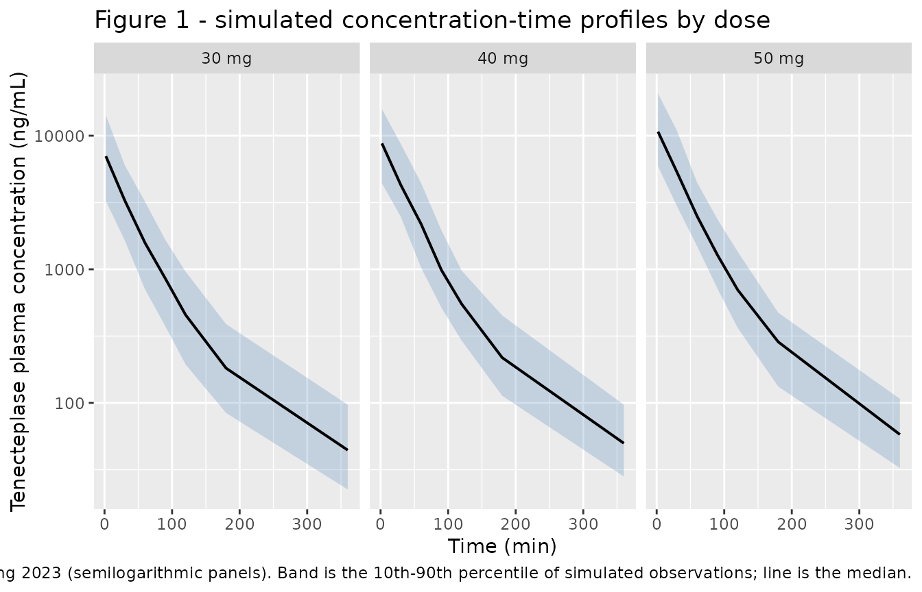
PKNCA validation
NCA is run on the typical-value reference-patient profiles at the
four dose levels the paper simulates, so the comparison against the
published dose/CL AUC values is exact rather than
cohort-dependent. Concentrations are tenecteplase-only (background
removed, as described above).
sim_nca <- sim_anchor |>
  dplyr::mutate(Cc = tnk_conc(sim_anchor)) |>
  dplyr::filter(!is.na(Cc)) |>
  dplyr::select(id, time, Cc, label)

# Guarantee a time = 0 row per (id, label). For an IV bolus the t = 0 record is
# the peak, which the solve already provides; this is a defensive no-op that
# keeps PKNCA from warning about an AUC range starting before the first
# measurement.
sim_nca <- dplyr::bind_rows(
  sim_nca,
  sim_nca |> dplyr::distinct(id, label) |> dplyr::mutate(time = 0, Cc = 0)
) |>
  dplyr::distinct(id, label, time, .keep_all = TRUE) |>
  dplyr::arrange(id, label, time)

conc_obj <- PKNCA::PKNCAconc(sim_nca, Cc ~ time | label + id)

dose_df <- anchors |>
  dplyr::mutate(time = 0) |>
  dplyr::select(id, time, amt, label)
dose_obj <- PKNCA::PKNCAdose(dose_df, amt ~ time | label + id)

intervals <- data.frame(
  start = 0, end = Inf,
  cmax = TRUE, tmax = TRUE, aucinf.obs = TRUE, half.life = TRUE
)

nca_res <- PKNCA::pk.nca(PKNCA::PKNCAdata(conc_obj, dose_obj, intervals = intervals))
knitr::kable(as.data.frame(nca_res), digits = 3,
caption = "PKNCA results for the typical-value reference patient at each simulated dose level.")| label | id | start | end | PPTESTCD | PPORRES | exclude |
|---|---|---|---|---|---|---|
| 0.1 mg/kg | 1 | 0 | Inf | cmax | 1939.058 | NA |
| 0.1 mg/kg | 1 | 0 | Inf | tmax | 0.000 | NA |
| 0.1 mg/kg | 1 | 0 | Inf | tlast | 1440.000 | NA |
| 0.1 mg/kg | 1 | 0 | Inf | clast.obs | 0.000 | NA |
| 0.1 mg/kg | 1 | 0 | Inf | lambda.z | 0.009 | NA |
| 0.1 mg/kg | 1 | 0 | Inf | r.squared | 1.000 | NA |
| 0.1 mg/kg | 1 | 0 | Inf | adj.r.squared | 1.000 | NA |
| 0.1 mg/kg | 1 | 0 | Inf | lambda.z.time.first | 208.000 | NA |
| 0.1 mg/kg | 1 | 0 | Inf | lambda.z.time.last | 1440.000 | NA |
| 0.1 mg/kg | 1 | 0 | Inf | lambda.z.n.points | 185.000 | NA |
| 0.1 mg/kg | 1 | 0 | Inf | clast.pred | 0.000 | NA |
| 0.1 mg/kg | 1 | 0 | Inf | half.life | 76.731 | NA |
| 0.1 mg/kg | 1 | 0 | Inf | span.ratio | 16.056 | NA |
| 0.1 mg/kg | 1 | 0 | Inf | aucinf.obs | 79715.539 | NA |
| 0.25 mg/kg | 2 | 0 | Inf | cmax | 4847.645 | NA |
| 0.25 mg/kg | 2 | 0 | Inf | tmax | 0.000 | NA |
| 0.25 mg/kg | 2 | 0 | Inf | tlast | 1440.000 | NA |
| 0.25 mg/kg | 2 | 0 | Inf | clast.obs | 0.001 | NA |
| 0.25 mg/kg | 2 | 0 | Inf | lambda.z | 0.009 | NA |
| 0.25 mg/kg | 2 | 0 | Inf | r.squared | 1.000 | NA |
| 0.25 mg/kg | 2 | 0 | Inf | adj.r.squared | 1.000 | NA |
| 0.25 mg/kg | 2 | 0 | Inf | lambda.z.time.first | 208.000 | NA |
| 0.25 mg/kg | 2 | 0 | Inf | lambda.z.time.last | 1440.000 | NA |
| 0.25 mg/kg | 2 | 0 | Inf | lambda.z.n.points | 185.000 | NA |
| 0.25 mg/kg | 2 | 0 | Inf | clast.pred | 0.001 | NA |
| 0.25 mg/kg | 2 | 0 | Inf | half.life | 76.731 | NA |
| 0.25 mg/kg | 2 | 0 | Inf | span.ratio | 16.056 | NA |
| 0.25 mg/kg | 2 | 0 | Inf | aucinf.obs | 199288.848 | NA |
| 0.5 mg/kg | 3 | 0 | Inf | cmax | 9695.291 | NA |
| 0.5 mg/kg | 3 | 0 | Inf | tmax | 0.000 | NA |
| 0.5 mg/kg | 3 | 0 | Inf | tlast | 1440.000 | NA |
| 0.5 mg/kg | 3 | 0 | Inf | clast.obs | 0.002 | NA |
| 0.5 mg/kg | 3 | 0 | Inf | lambda.z | 0.009 | NA |
| 0.5 mg/kg | 3 | 0 | Inf | r.squared | 1.000 | NA |
| 0.5 mg/kg | 3 | 0 | Inf | adj.r.squared | 1.000 | NA |
| 0.5 mg/kg | 3 | 0 | Inf | lambda.z.time.first | 208.000 | NA |
| 0.5 mg/kg | 3 | 0 | Inf | lambda.z.time.last | 1440.000 | NA |
| 0.5 mg/kg | 3 | 0 | Inf | lambda.z.n.points | 185.000 | NA |
| 0.5 mg/kg | 3 | 0 | Inf | clast.pred | 0.002 | NA |
| 0.5 mg/kg | 3 | 0 | Inf | half.life | 76.731 | NA |
| 0.5 mg/kg | 3 | 0 | Inf | span.ratio | 16.056 | NA |
| 0.5 mg/kg | 3 | 0 | Inf | aucinf.obs | 398577.694 | NA |
| 50 mg | 4 | 0 | Inf | cmax | 11852.434 | NA |
| 50 mg | 4 | 0 | Inf | tmax | 0.000 | NA |
| 50 mg | 4 | 0 | Inf | tlast | 1440.000 | NA |
| 50 mg | 4 | 0 | Inf | clast.obs | 0.002 | NA |
| 50 mg | 4 | 0 | Inf | lambda.z | 0.009 | NA |
| 50 mg | 4 | 0 | Inf | r.squared | 1.000 | NA |
| 50 mg | 4 | 0 | Inf | adj.r.squared | 1.000 | NA |
| 50 mg | 4 | 0 | Inf | lambda.z.time.first | 208.000 | NA |
| 50 mg | 4 | 0 | Inf | lambda.z.time.last | 1440.000 | NA |
| 50 mg | 4 | 0 | Inf | lambda.z.n.points | 185.000 | NA |
| 50 mg | 4 | 0 | Inf | clast.pred | 0.002 | NA |
| 50 mg | 4 | 0 | Inf | half.life | 76.731 | NA |
| 50 mg | 4 | 0 | Inf | span.ratio | 16.056 | NA |
| 50 mg | 4 | 0 | Inf | aucinf.obs | 487258.794 | NA |
Comparison against published NCA
The paper does not tabulate a conventional NCA table; the only
exposure metric it publishes is AUC derived as dose/CL.
Those are the reference values below, converted to
ng*min/mL to match PKNCA’s units. The 0.25 mg/kg level has
no published point estimate (only a 90% prediction interval) and so is
excluded from this table.
published <- tibble::tribble(
  ~label,       ~aucinf.obs,
  "0.1 mg/kg",   79.7 * 1000,
  "0.5 mg/kg",  398   * 1000,
  "50 mg",      487   * 1000
)

cmp <- nlmixr2lib::ncaComparisonTable(
  simulated     = nca_res,
  reference     = published,
  by            = "label",
  params        = "aucinf.obs",
  units         = c(aucinf.obs = "ng*min/mL"),
  tolerance_pct = 20
)

knitr::kable(cmp,
caption = "Simulated (PKNCA, aucinf.obs) vs published AUC = dose/CL. * differs from reference by >20%.")| NCA parameter | label | Reference | Simulated | % diff |
|---|---|---|---|---|
| AUC0-∞ (obs) (ng*min/mL) | 0.1 mg/kg | 79700 | 79700 | +0.0% |
| AUC0-∞ (obs) (ng*min/mL) | 0.5 mg/kg | 398000 | 399000 | +0.1% |
| AUC0-∞ (obs) (ng*min/mL) | 50 mg | 487000 | 487000 | +0.1% |
# Independent of the display table: PKNCA's AUCinf must agree with the
# published dose/CL values. Deterministic typical-value profiles.
nca_auc <- as.data.frame(nca_res) |>
  dplyr::filter(PPTESTCD == "aucinf.obs") |>
  dplyr::select(label, PPORRES) |>
  dplyr::left_join(published, by = "label") |>
  dplyr::filter(!is.na(aucinf.obs)) |>
  dplyr::mutate(pct_diff = 100 * (PPORRES - aucinf.obs) / aucinf.obs)

stopifnot(nrow(nca_auc) == 3L)               # the gate must have rows to test
print(nca_auc)
#> # A tibble: 3 × 4
#>   label     PPORRES aucinf.obs pct_diff
#>   <chr>       <dbl>      <dbl>    <dbl>
#> 1 0.1 mg/kg  79716.      79700   0.0195
#> 2 0.5 mg/kg 398578.     398000   0.145
#> 3 50 mg     487259.     487000   0.0531
stopifnot(max(abs(nca_auc$pct_diff)) < 2)
External validation against study N1811s
The paper’s partial external validation compares model predictions against summary statistics from 75 patients with acute ischemic stroke (study N1811s), sampled once at 1 hour post dose. Observed means (SD) were 389 (146), 641 (240), 1227 (491) and 1647 (732) ng/mL at 0.1, 0.2, 0.4 and 0.5 mg/kg. The paper reports that the model overpredicted these means by a factor of about 1.39 on average, while 71.7% of the derived observation distribution still fell inside the model’s 90% prediction interval.
This replication is approximate by construction: N1811s reported neither weight nor CRCL-NM, so the authors assumed the TIMI 10B weight distribution and predicted CRCL-NM from each group’s median age using an age/CRCL-NM regression fitted to TIMI 10B that the paper does not report. The cohort below therefore uses the TIMI 10B covariate distribution unchanged for both. Because the stroke population is older with lower renal function, the paper’s own simulation sits somewhat higher than this one.
set.seed(18110)
rxode2::rxSetSeed(18110)

n1811s_obs <- tibble::tribble(
  ~arm,          ~dose_mgkg, ~obs_mean,
  "0.1 mg/kg",   0.1,         389,
  "0.2 mg/kg",   0.2,         641,
  "0.4 mg/kg",   0.4,        1227,
  "0.5 mg/kg",   0.5,        1647
)

make_wb_cohort <- function(n, dose_mgkg, arm, id_offset) {
  subj <- tibble::tibble(
    id   = id_offset + seq_len(n),
    WT   = pmin(pmax(stats::rnorm(n, 84.1, 20.0), 45), 150),
    CRCL = pmin(pmax(stats::rnorm(n, 83.3, 25.5), 20), 170),
    arm  = arm
  ) |>
    dplyr::mutate(amt = dose_mgkg * WT)
  dose <- subj |> dplyr::mutate(time = 0, evid = 1L, cmt = "central")
  obs  <- subj |> dplyr::mutate(time = 60, amt = NA_real_, evid = 0L, cmt = "central")
  dplyr::bind_rows(dose, obs) |> dplyr::arrange(id, time, dplyr::desc(evid))
}

ev_n1811s <- dplyr::bind_rows(
  lapply(seq_len(nrow(n1811s_obs)), function(i) {
    make_wb_cohort(150L, n1811s_obs$dose_mgkg[i], n1811s_obs$arm[i],
                   id_offset = i * 10000L)
  })
)
stopifnot(!anyDuplicated(unique(ev_n1811s[, c("id", "time", "evid")])))

sim_n1811s <- rxode2::rxSolve(mod, events = ev_n1811s,
                              keep = c("WT", "CRCL", "arm"),
                              returnType = "data.frame")

ext <- sim_n1811s |>
  dplyr::filter(time == 60) |>
  dplyr::group_by(arm) |>
  dplyr::summarise(model_mean = mean(sim), .groups = "drop") |>
  dplyr::left_join(n1811s_obs, by = "arm") |>
  dplyr::mutate(ratio = model_mean / obs_mean)

ext |>
  dplyr::select(arm, obs_mean, model_mean, ratio) |>
  dplyr::rename("Dose" = arm,
                "Observed mean (ng/mL)" = obs_mean,
                "Model mean (ng/mL)"    = model_mean,
                "Model / observed"      = ratio) |>
  knitr::kable(digits = c(0, 0, 0, 2),
caption = "External validation against study N1811s at 1 hour post dose. Tang 2023 reports a mean overprediction factor of about 1.39.")| Dose | Observed mean (ng/mL) | Model mean (ng/mL) | Model / observed |
|---|---|---|---|
| 0.1 mg/kg | 389 | 480 | 1.23 |
| 0.2 mg/kg | 641 | 1025 | 1.60 |
| 0.4 mg/kg | 1227 | 1800 | 1.47 |
| 0.5 mg/kg | 1647 | 2283 | 1.39 |
# The direction and rough magnitude of the overprediction are the published
# claim; the exact factor depends on the unreported age/CRCL-NM regression, and
# a mean over a heavy-tailed lognormal residual (omega 0.789 on the residual
# magnitude) is itself a noisy statistic. The bound is wide enough to survive
# any cohort the model can draw while still failing on a unit or dose error,
# which would move the ratio by an order of magnitude.
stopifnot(median(ext$ratio) > 1.0, median(ext$ratio) < 2.5)
Assumptions and deviations
-
Variance scale. Table 1’s “CV” column is read as
omega standard deviations, on the strength of the Table
S3/S4 caption (“The RSE for IIV and RUV parameters is reported on the
approximate SD scale”) and the log-additive residual row. If the column
instead held
sqrt(exp(omega^2) - 1), the structural IIVs would change by under 2% and the IIV on the residual magnitude by about 12%; no published quantity in the paper resolves it more tightly than the caption already does. -
IIV on Vc is not separately reported. The paper
estimates a single eta shared by CL and Vc with a scaler (correlation
fixed to 1). The implied omega for Vc is
0.913 * 0.199= 0.182 and is not printed anywhere in the paper. -
Alternative covariate model not encoded. Run 50
(age and race on CL, Table S4) is a sensitivity analysis with a worse
OFV than the final model; only the final model (run 34) is packaged. Age
and race are recorded in
covariatesDataExcludedwith their run-50 coefficients so the provenance is preserved. -
Background signal in
Cc.Ccis the assay-measured total, i.e. tenecteplase plus the endogenous t-PA background (Eq. 2), following theBauer_2023_vonicogAlfa.Rconvention. The background is removed before NCA and before every AUC integration in this vignette, because the paper’s AUC isdose/CL(tenecteplase only). Setbl_tpato zero to recover the tenecteplase-only prediction directly. - Virtual cohort covariates. Weight and CRCL-NM are drawn independently from normal distributions matched to the Table S1 means and SDs and truncated to physiological ranges. The paper reports these marginally, not jointly, and Figure S2 shows they are correlated with age and each other; the independence assumption is a simplification and affects only the cohort figures, not the deterministic checks.
- N1811s external validation is approximate. Neither weight nor CRCL-NM was reported for N1811s. The paper predicted CRCL-NM from median age via a TIMI 10B regression that it does not publish; this vignette instead reuses the TIMI 10B covariate distribution. The reproduced overprediction is therefore expected to differ somewhat from the paper’s stated factor of 1.39, and the assertion is correspondingly wide.
- No published NCA table. The paper reports no Cmax / Tmax / half-life values, so the NCA comparison covers AUC only. The other PKNCA parameters are shown for completeness but have no published counterpart.
- All parameter values come from the paper’s own text, Table 1 and the open-access supplement (Tables S1-S4). No value was digitized from a figure, supplied by correspondence, or carried from an upstream model.