Model and source
- Citation: Zhang Y, Mai H, Guo G, Bi G, Hao G, Li Y, Wang X, Cheng L, Wang J, Dong R, Liu Z, Chen L, Qu H (2018). Association analysis of SNPs present in plasma with adverse events and population pharmacokinetics in Chinese sunitinib treated patients with renal cell carcinoma. Oncotarget 9(18):14109-14123. doi:10.18632/oncotarget.23881.
- Description: One-compartment parent-plus-metabolite population PK model for oral sunitinib and its active metabolite N-desethyl sunitinib (SU12662) in 53 Chinese patients with renal-cell carcinoma dosed on the 4-weeks-on / 2-weeks-off schedule (Zhang 2018). Sunitinib is absorbed first order into a single central compartment and eliminated with apparent oral clearance Clp/F; that elimination flux is the sole input to a single SU12662 compartment, which is eliminated with apparent clearance Clm/F. Because only oral data were available, the fraction of sunitinib converted to SU12662 is not identifiable and is folded into the apparent metabolite clearance and volume, so the metabolite parameters are apparent values conditioned on complete conversion. Sunitinib and SU12662 were fitted simultaneously in Phoenix NLME. Body weight (power 0.538, reference 68.3 kg) and the ABCB1 rs2032582 genotype entered as a six-level linear proportional effect (AT reference) on Clm/F only; the paper reports that no covariate (weight, age, sex or genotype) was retained on the parent Clp/F or V/F. Inter-individual variability was estimated (eta shrinkages are tabulated) but no omega values were published, so every eta is carried at fixed(0); residual error is combined proportional plus additive, reported separately for sunitinib and SU12662.
- Article: https://doi.org/10.18632/oncotarget.23881
Zhang 2018 is primarily a pharmacogenomic association study: it genotyped eight SNPs in six candidate genes from cell-free plasma DNA and related them to sunitinib treatment-emergent adverse events in Chinese patients with renal-cell carcinoma. The population PK model extracted here is the paper’s final quantitative model, fitted simultaneously to sunitinib and its active metabolite N-desethyl sunitinib (SU12662), with the ABCB1 rs2032582 genotype retained as a predictive covariate on the apparent clearance of SU12662.
Population
Fifty-three patients with histologically confirmed renal-cell carcinoma were enrolled at the Academy of Military Medical Sciences Affiliated Hospital (Beijing) between March 2014 and January 2016, contributing 127 plasma samples (Table 1 and Results). Forty (75.5%) were male, the median age was 54 years (range 19-71; Table 1 reports 51.65 years with quartiles 45-61), and median body surface area was 1.86 m2 (quartiles 1.74-1.94). All subjects were Chinese. Forty (75.5%) had undergone a prior nephrectomy; ECOG performance status was 0 in 37 and 1 in 16 subjects.
Sunitinib was given orally as a single agent, 50 mg once daily for four weeks followed by two weeks off (schedule 4/2), with protocol-permitted reductions for toxicity. Over the first four cycles the daily dose was 50 mg in 64.2%, 37.5 mg in 15.1% and 25 mg in 20.8% of subjects; 35.9% had a dose reduction after cycle 1, 2 or 3 (Table 1). PK samples were drawn on day 15 +/- 1, after the steady state the authors considered established at 14 days.
The paper does not tabulate body weight, but states a cohort average of 68.3 kg in Methods (equation 4), which is the reference weight of the covariate model.
The same information is available programmatically via
readModelDb("Zhang_2018_sunitinib")()$population.
Source trace
Every ini() entry in
inst/modeldb/specificDrugs/Zhang_2018_sunitinib.R carries
an in-file comment pointing at its origin. They are collected here for
review.
| Equation / parameter | Value | Source location |
|---|---|---|
lka (ka) |
0.0117 1/h | Table 6, final model, tvKa
|
lvc (V/F, sunitinib) |
99438 mL | Table 6, final model, tvV
|
lcl (Clp/F, sunitinib) |
24576 mL/h | Table 6, final model, tvClp
|
lvc_su12662 (V2/F, SU12662) |
916641 mL | Table 6, final model, tvV2
|
lcl_su12662 (Clm/F, SU12662) |
53614 mL/h | Table 6, final model, tvClm; also the intercept of the
“final equation” (p. 14114) |
e_wt_cl_su12662 |
0.538 | Table 6, dClmdBW; reference weight 68.3 kg from Methods
equation 4 |
e_snp_abcb1_rs2032582_tg_cl_su12662 |
0.314 | Table 6, dClmdZ31; final equation term
(1 - 0.314 * (Z3 = 1))
|
e_snp_abcb1_rs2032582_gg_cl_su12662 |
0.269 | Table 6, dClmdZ32; final equation term
(1 - 0.269 * (Z3 = 2))
|
e_snp_abcb1_rs2032582_tt_cl_su12662 |
0.308 | Table 6, dClmdZ33; final equation term
(1 - 0.308 * (Z3 = 3))
|
e_snp_abcb1_rs2032582_ag_cl_su12662 |
0.0368 | Table 6, dClmdZ34; final equation term
(1 - 0.0368 * (Z3 = 4))
|
e_snp_abcb1_rs2032582_gt_cl_su12662 |
0.0456 | Table 6, dClmdZ35; final equation term
(1 - 0.0456 * (Z3 = 5))
|
propSd (sunitinib) |
0.31 | Table 6, final model, tvCMultStdev
|
addSd (sunitinib) |
0.0751 ng/mL | Table 6, final model, stdev0
|
propSd_su12662 |
0.242 | Table 6, final model, tvC2MultStdev
|
addSd_su12662 |
1.23 ng/mL | Table 6, final model, stdev1
|
etalka, etalvc, etalcl,
etalvc_su12662, etalcl_su12662
|
fixed(0) |
Table 6 reports eta shrinkage (0.386 / 0.773 / 0.317 / 0.975 / 0.163) but no omega anywhere in the paper; see Assumptions and deviations |
d/dt(depot), d/dt(central)
|
n/a | Results: “a one-compartment model with first-order adsorption”; Supplementary Figure 1 schematic (not obtainable, see Errata) |
d/dt(central_su12662) |
n/a | Results: “Sunitinib and SU12662 were modeled simultaneously”; final-equation footnote “m represent for the metabolite SU12662” |
| Covariate model form | n/a | Methods “Model development”, equations 2 and 4; final equation p. 14114 |
| Residual-error form | n/a | Methods “Model development”, equation 3 |
mod <- readModelDb("Zhang_2018_sunitinib")
ui <- rxode2::rxode(mod)
#> ℹ parameter labels from comments will be replaced by 'label()'
ui$state
#> [1] "depot"           "central"         "central_su12662"
Structural checks
These checks are deterministic: a single typical subject, no random effects, no cohort. They therefore hold on any machine and at any solver-thread count, and they are the checks that actually pin the structure.
# Observation grid: coarse across the 28-day on-period, dense over the two
# dosing intervals that are compared against the paper (day 15, the paper's
# sampling day, and day 28, the end of the on-period).
DAY15 <- c(336, 360)
DAY28 <- c(648, 672)
OBS_TIMES <- sort(unique(c(
  seq(0, 672, by = 24),
  seq(DAY15[1], DAY15[2], by = 1),
  seq(DAY28[1], DAY28[2], by = 1)
)))

GENOTYPES <- c("AT", "TG", "GG", "TT", "AG", "GT")

# Zhang 2018 codes the ABCB1 rs2032582 genotype as a single six-level variable
# Z3 (0 = AT, 1 = TG, 2 = GG, 3 = TT, 4 = AG, 5 = GT). nlmixr2lib encodes it as
# five binary indicators with AT (all indicators zero) as the reference.
geno_indicators <- function(genotype) {
  stopifnot(all(genotype %in% GENOTYPES))
  tibble::tibble(
    SNP_ABCB1_RS2032582_TG = as.numeric(genotype == "TG"),
    SNP_ABCB1_RS2032582_GG = as.numeric(genotype == "GG"),
    SNP_ABCB1_RS2032582_TT = as.numeric(genotype == "TT"),
    SNP_ABCB1_RS2032582_AG = as.numeric(genotype == "AG"),
    SNP_ABCB1_RS2032582_GT = as.numeric(genotype == "GT")
  )
}

# One cohort as a self-contained event table. `id_offset` keeps IDs disjoint
# when several cohorts are bind_rows()-ed; duplicate IDs are silently merged by
# rxSolve into a single subject receiving the summed dose.
make_cohort <- function(dose_mg, WT, genotype, id_offset = 0L) {
  n <- max(length(WT), length(genotype))
  subj <- tibble::tibble(
    id = id_offset + seq_len(n),
    WT = rep(WT, length.out = n),
    genotype = rep(genotype, length.out = n),
    dose_mg = dose_mg,
    treatment = paste(format(dose_mg, trim = TRUE), "mg")
  )
  subj <- dplyr::bind_cols(subj, geno_indicators(subj$genotype))

  dose <- subj |>
    dplyr::mutate(
      time = 0, amt = dose_mg, cmt = "depot", evid = 1L,
      ii = 24, addl = 27L, dvid = NA_integer_
    )
  # cmt on observation rows is the ODE state, never the observable name; with
  # two endpoints, dvid = 1 on every observation row makes rxode2 return every
  # derived variable (Cc and Cc_su12662) as wide columns from one solve.
  obs <- subj |>
    tidyr::crossing(time = OBS_TIMES) |>
    dplyr::mutate(
      amt = NA_real_, cmt = "central", evid = 0L,
      ii = 0, addl = 0L, dvid = 1L
    )
  dplyr::bind_rows(dose, obs) |>
    dplyr::arrange(id, time, dplyr::desc(evid))
}

# useLinCmt = FALSE: rxode2's automatic ODE -> linCmt conversion recognises the
# ka / cl / vc triple and can solve the parent analytically, which would drop
# the metabolite state from the system entirely. The first assertion below is
# the gate on exactly that.
solve_model <- function(events, params = NULL, ...) {
  rxode2::rxSolve(
    mod, events,
    useLinCmt = FALSE, returnType = "data.frame",
    params = params, ...
  )
}
ev_typ <- make_cohort(dose_mg = 50, WT = 68.3, genotype = "AT")
sim_typ <- solve_model(ev_typ)
#> ℹ parameter labels from comments will be replaced by 'label()'
#> ℹ omega/sigma items treated as zero: 'etalka', 'etalvc', 'etalcl', 'etalvc_su12662', 'etalcl_su12662'

# Every declared ODE state must appear in the solve output. If rxode2 had
# auto-solved the parent analytically, central_su12662 would be absent and the
# model would silently be a one-analyte model.
stopifnot(all(ui$state %in% names(sim_typ)))
stopifnot("central_su12662" %in% names(sim_typ))
ui$state
#> [1] "depot"           "central"         "central_su12662"
# The paper's "final equation", transcribed independently of the model file.
paper_clm <- function(WT, genotype) {
  53614 * (WT / 68.3)^0.538 *
    (1 - 0.314 * (genotype == "TG")) *
    (1 - 0.269 * (genotype == "GG")) *
    (1 - 0.308 * (genotype == "TT")) *
    (1 - 0.0368 * (genotype == "AG")) *
    (1 - 0.0456 * (genotype == "GT"))
}

grid <- tidyr::crossing(WT = c(50, 68.3, 90), genotype = GENOTYPES)
ev_grid <- make_cohort(dose_mg = 50, WT = grid$WT, genotype = grid$genotype)
sim_grid <- solve_model(ev_grid, keep = c("WT", "genotype"))
#> ℹ omega/sigma items treated as zero: 'etalka', 'etalvc', 'etalcl', 'etalvc_su12662', 'etalcl_su12662'
#> Warning: multi-subject simulation without without 'omega'

clm_check <- sim_grid |>
  dplyr::distinct(id, WT, genotype, cl_su12662) |>
  dplyr::mutate(paper = paper_clm(WT, genotype),
                rel_diff = abs(cl_su12662 / paper - 1))

# Deterministic: the model must reproduce the printed equation to machine
# precision, not approximately.
stopifnot(nrow(clm_check) == nrow(grid))
stopifnot(max(clm_check$rel_diff) < 1e-10)
# ... and the AT reference subject at the reference weight must be the
# tabulated Clm/F intercept exactly.
stopifnot(
  abs(clm_check$cl_su12662[clm_check$WT == 68.3 & clm_check$genotype == "AT"] / 53614 - 1) < 1e-10
)

clm_check |>
  dplyr::filter(WT == 68.3) |>
  dplyr::mutate(
    ratio_to_AT = cl_su12662 / cl_su12662[genotype == "AT"],
    genotype = factor(genotype, levels = GENOTYPES)
  ) |>
  dplyr::arrange(genotype) |>
  dplyr::transmute(
    "rs2032582 genotype" = genotype,
    "Clm/F (mL/h)" = round(cl_su12662, 1),
    "Ratio to AT reference" = round(ratio_to_AT, 4)
  ) |>
knitr::kable(caption = "SU12662 apparent clearance by ABCB1 rs2032582 genotype at the 68.3 kg reference weight (reproduces the final equation on p. 14114).")| rs2032582 genotype | Clm/F (mL/h) | Ratio to AT reference |
|---|---|---|
| AT | 53614.0 | 1.0000 |
| TG | 36779.2 | 0.6860 |
| GG | 39191.8 | 0.7310 |
| TT | 37100.9 | 0.6920 |
| AG | 51641.0 | 0.9632 |
| GT | 51169.2 | 0.9544 |
# The metabolite arm must be live and the flow must be one-way. Doubling Clm/F
# has to move SU12662 substantially and must not touch sunitinib at all.
sim_pert <- solve_model(ev_typ, params = c(lcl_su12662 = log(2 * 53614)))
#> ℹ omega/sigma items treated as zero: 'etalka', 'etalvc', 'etalcl', 'etalvc_su12662', 'etalcl_su12662'

ss <- sim_typ$time >= DAY28[1]
rel_m <- max(abs(sim_pert$Cc_su12662[ss] / sim_typ$Cc_su12662[ss] - 1))
rel_p <- max(abs(sim_pert$Cc[ss] / sim_typ$Cc[ss] - 1))

stopifnot(rel_m > 0.3)   # metabolite responds (halving of exposure is expected)
stopifnot(rel_p < 1e-8)  # parent is unaffected: conversion is unidirectional
c(metabolite_relative_change = rel_m, parent_relative_change = rel_p)
#> metabolite_relative_change     parent_relative_change
#>               5.077542e-01               6.217249e-15
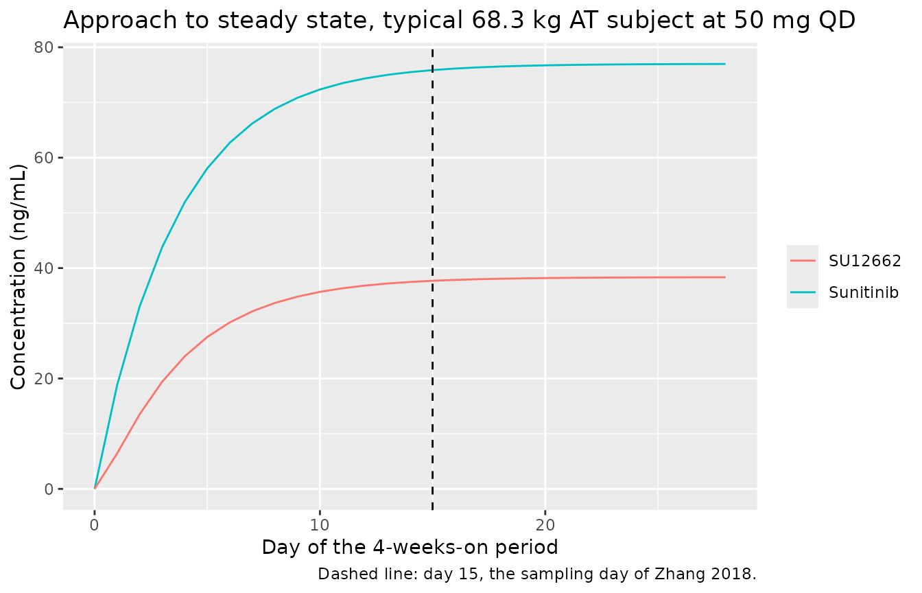
The model’s absorption rate constant (0.0117 1/h, an absorption
half-life of 59 h) is far slower than the parent’s disposition
(cl / vc gives a half-life of about 2.8 h), so the system
is absorption-limited: the observable decline is governed by
ka, and steady state is approached on the absorption time
scale. That is self-consistent with the authors’ design, which sampled
on day 15 because they considered steady state reached at 14 days.
approach <- sim_typ |>
  dplyr::filter(time %in% seq(0, 672, by = 24)) |>
  dplyr::transmute(day = time / 24, Cc, Cc_su12662)

# Fraction of the eventual steady-state trough reached at day 15, predicted
# analytically from ka alone.
frac_day15 <- 1 - exp(-0.0117 * 360)
stopifnot(frac_day15 > 0.95)
round(frac_day15, 4)
#> [1] 0.9852

ggplot(approach, aes(day)) +
  geom_line(aes(y = Cc, colour = "Sunitinib")) +
  geom_line(aes(y = Cc_su12662, colour = "SU12662")) +
  geom_vline(xintercept = 15, linetype = "dashed") +
  labs(
    x = "Day of the 4-weeks-on period", y = "Concentration (ng/mL)",
    colour = NULL,
    title = "Approach to steady state, typical 68.3 kg AT subject at 50 mg QD",
    caption = "Dashed line: day 15, the sampling day of Zhang 2018."
  )
Virtual cohort
Original observed data are not publicly available. The cohort below matches the published dose groups (Table 1: 50, 37.5 and 25 mg daily over the first four cycles) at 100 subjects per arm.
Zhang 2018 reports no body-weight distribution, only the 68.3 kg
cohort average used as the covariate reference. Weight is therefore
drawn from a normal distribution centred on that average and truncated
to a plausible adult range; this is an assumption, recorded below. All
cohort subjects carry the AT reference genotype, because
the six-level Z3 frequencies are not recoverable from the paper (Table 2
pools the genotypes into three association-analysis strata that do not
match the model’s coding). The genotype effect is shown
deterministically in the structural checks above instead.
# set.seed() seeds R's RNG for the weight draw. It does NOT seed rxode2's
# simulation RNG; here that is immaterial because every eta is fixed(0), so the
# model has no between-subject random effects at all and the only source of
# variability below is the drawn weight.
set.seed(20180306)

N_PER_ARM <- 100L
draw_weight <- function(n) pmin(pmax(rnorm(n, mean = 68.3, sd = 10), 45), 95)

events <- dplyr::bind_rows(
  make_cohort(25, draw_weight(N_PER_ARM), "AT", id_offset = 0L),
  make_cohort(37.5, draw_weight(N_PER_ARM), "AT", id_offset = 100L),
  make_cohort(50, draw_weight(N_PER_ARM), "AT", id_offset = 200L)
)
stopifnot(!anyDuplicated(unique(events[, c("id", "time", "evid")])))
stopifnot(dplyr::n_distinct(events$id) == 3L * N_PER_ARM)
Simulation
sim <- solve_model(events, keep = c("treatment", "dose_mg", "WT", "genotype"))
#> ℹ omega/sigma items treated as zero: 'etalka', 'etalvc', 'etalcl', 'etalvc_su12662', 'etalcl_su12662'
#> Warning: multi-subject simulation without without 'omega'
if (is.null(sim$id)) sim$id <- 1L
stopifnot(all(ui$state %in% names(sim)))
stopifnot(!anyNA(sim$Cc), !anyNA(sim$Cc_su12662))
Replicate published figures
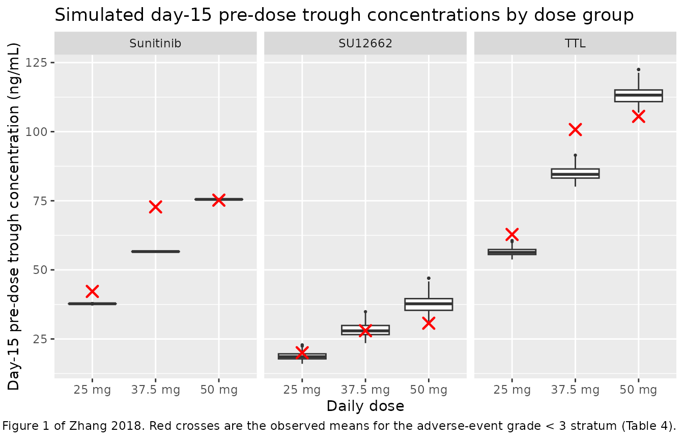
Figure 1 of Zhang 2018 plots the steady-state plasma concentration of sunitinib, of SU12662, and of their sum (the “total trough level”, TTL) for all treated patients, with the median marked. The figure itself shows individual observed points, which are not available; the panel below shows the corresponding simulated day-15 distributions by dose group, with the paper’s reported group means (Table 4, adverse-event grade < 3 rows) overlaid.
day15 <- sim |>
  dplyr::filter(time == DAY15[1]) |>
  dplyr::transmute(
    id, treatment, WT,
    Sunitinib = Cc, SU12662 = Cc_su12662, TTL = Cc + Cc_su12662
  ) |>
  tidyr::pivot_longer(c(Sunitinib, SU12662, TTL),
    names_to = "analyte", values_to = "conc"
  ) |>
  dplyr::mutate(
    analyte = factor(analyte, levels = c("Sunitinib", "SU12662", "TTL")),
    treatment = factor(treatment, levels = c("25 mg", "37.5 mg", "50 mg"))
  )

published_mean <- tibble::tribble(
  ~treatment, ~analyte, ~conc,
  "25 mg", "TTL", 62.81,
  "37.5 mg", "TTL", 100.76,
  "50 mg", "TTL", 105.53,
  "25 mg", "Sunitinib", 42.20,
  "37.5 mg", "Sunitinib", 72.78,
  "50 mg", "Sunitinib", 75.22,
  "25 mg", "SU12662", 20.02,
  "37.5 mg", "SU12662", 27.99,
  "50 mg", "SU12662", 30.70
) |>
  dplyr::mutate(
    analyte = factor(analyte, levels = c("Sunitinib", "SU12662", "TTL")),
    treatment = factor(treatment, levels = c("25 mg", "37.5 mg", "50 mg"))
  )

ggplot(day15, aes(treatment, conc)) +
  geom_boxplot(outlier.size = 0.5) +
  geom_point(
    data = published_mean, aes(treatment, conc),
    colour = "red", shape = 4, size = 3, stroke = 1.2
  ) +
  facet_wrap(~analyte) +
  labs(
    x = "Daily dose", y = "Day-15 pre-dose trough concentration (ng/mL)",
    title = "Simulated day-15 pre-dose trough concentrations by dose group",
    caption = paste(
      "Corresponds to Figure 1 of Zhang 2018. Red crosses are the observed",
      "means for the adverse-event grade < 3 stratum (Table 4)."
    )
  )
PKNCA validation
NCA is run at steady state over the day-15 dosing interval (the paper’s sampling day) and over the day-28 interval (the end of the 4-weeks-on period, where the approach to steady state is essentially complete). Sunitinib, SU12662 and their sum are treated as three analytes within one PKNCA object so a single combined comparison table can be rendered.
sim_nca <- sim |>
  dplyr::filter(!is.na(Cc)) |>
  dplyr::transmute(
    id, time, treatment,
    Sunitinib = Cc, SU12662 = Cc_su12662, TTL = Cc + Cc_su12662
  ) |>
  tidyr::pivot_longer(c(Sunitinib, SU12662, TTL),
    names_to = "analyte", values_to = "Cc"
  )

# Guarantee a time = 0 record per (id, treatment, analyte). Sunitinib is given
# orally, so the pre-dose concentration is zero.
sim_nca <- dplyr::bind_rows(
  sim_nca,
  sim_nca |>
    dplyr::distinct(id, treatment, analyte) |>
    dplyr::mutate(time = 0, Cc = 0)
) |>
  dplyr::distinct(id, treatment, analyte, time, .keep_all = TRUE) |>
  dplyr::arrange(id, treatment, analyte, time)

dose_df <- events |>
  dplyr::filter(evid == 1) |>
  dplyr::select(id, time, amt, treatment) |>
  tidyr::crossing(analyte = c("Sunitinib", "SU12662", "TTL"))

conc_obj <- PKNCA::PKNCAconc(
  as.data.frame(sim_nca), Cc ~ time | treatment + analyte + id,
  concu = "ng/mL", timeu = "h"
)
dose_obj <- PKNCA::PKNCAdose(
  as.data.frame(dose_df), amt ~ time | treatment + analyte + id,
  doseu = "mg"
)

intervals <- data.frame(
  start = c(DAY15[1], DAY28[1]),
  end = c(DAY15[2], DAY28[2]),
  cmax = TRUE, tmax = TRUE, cmin = TRUE,
  cav = TRUE, auclast = TRUE
)

nca_res <- PKNCA::pk.nca(PKNCA::PKNCAdata(conc_obj, dose_obj, intervals = intervals))
nca_tbl <- as.data.frame(nca_res$result)
stopifnot(nrow(nca_tbl) > 0)
Steady-state mass balance
At steady state on a fixed regimen, the amount cleared over one
dosing interval equals the amount delivered over it. For the parent this
is the standard CL/F * AUCtau = Dose identity. For the
metabolite the same identity holds only because the model
routes the entire parent elimination flux into the SU12662 compartment,
so this second check is what pins the coupling between the two analytes
– an AUC recovery check on the parent alone is blind to
it.
auc_ss <- nca_tbl |>
  dplyr::filter(PPTESTCD == "auclast", start == DAY28[1]) |>
  dplyr::select(id, treatment, analyte, auc = PPORRES)

mb <- sim |>
  dplyr::distinct(id, treatment, dose_mg, cl, cl_su12662) |>
  dplyr::inner_join(auc_ss, by = c("id", "treatment")) |>
  dplyr::filter(analyte != "TTL") |>
  dplyr::mutate(
    clearance = ifelse(analyte == "Sunitinib", cl, cl_su12662),
    # clearance (mL/h) * AUCtau (ng/mL * h) = ng cleared; dose in mg = 1e6 ng.
    recovered = clearance * auc / (dose_mg * 1e6)
  )

stopifnot(nrow(mb) == 2L * 3L * N_PER_ARM)
stopifnot(max(abs(mb$recovered - 1)) < 0.01)

mb |>
  dplyr::group_by(analyte) |>
  dplyr::summarise(
    "Min fraction recovered" = round(min(recovered), 4),
    "Median fraction recovered" = round(median(recovered), 4),
    "Max fraction recovered" = round(max(recovered), 4),
    .groups = "drop"
  ) |>
  dplyr::rename(Analyte = analyte) |>
knitr::kable(caption = "Steady-state mass balance over the day-28 dosing interval: clearance * AUCtau divided by the administered dose.")| Analyte | Min fraction recovered | Median fraction recovered | Max fraction recovered |
|---|---|---|---|
| SU12662 | 0.9995 | 0.9995 | 0.9995 |
| Sunitinib | 0.9994 | 0.9994 | 0.9994 |
Comparison against published concentrations
Zhang 2018 reports no NCA table. What it does report is the
steady-state trough concentration of each analyte by dose group and
adverse-event severity (Table 4), which corresponds to PKNCA’s
cmin over the day-15 dosing interval. That interval starts
at t = 336 h, i.e. after 14 complete days of dosing, so its minimum is
the pre-dose trough on day 15 – exactly the sample Zhang 2018 drew. The
reference values below are the grade < 3 rows, which are the
comparator stratum in the paper’s own t-tests.
published <- tibble::tribble(
  ~treatment, ~analyte, ~cmin,
  "25 mg", "Sunitinib", 42.20,
  "37.5 mg", "Sunitinib", 72.78,
  "50 mg", "Sunitinib", 75.22,
  "25 mg", "SU12662", 20.02,
  "37.5 mg", "SU12662", 27.99,
  "50 mg", "SU12662", 30.70,
  "25 mg", "TTL", 62.81,
  "37.5 mg", "TTL", 100.76,
  "50 mg", "TTL", 105.53
)

cmp <- nlmixr2lib::ncaComparisonTable(
  simulated = nca_tbl |> dplyr::filter(start == DAY15[1]),
  reference = published,
  by = c("treatment", "analyte"),
  units = c(cmin = "ng/mL"),
  tolerance_pct = 20
)

knitr::kable(
  cmp,
  caption = "Simulated day-15 pre-dose trough vs. the observed means of Zhang 2018 Table 4 (adverse-event grade < 3). * differs from the reference by more than 20%."
)| NCA parameter | treatment | analyte | Reference | Simulated | % diff |
|---|---|---|---|---|---|
| Cmin (ng/mL) | 25 mg | Sunitinib | 42.2 | 37.7 | -10.6% |
| Cmin (ng/mL) | 25 mg | SU12662 | 20 | 18.5 | -7.5% |
| Cmin (ng/mL) | 25 mg | TTL | 62.8 | 56.3 | -10.3% |
| Cmin (ng/mL) | 37.5 mg | Sunitinib | 72.8 | 56.6 | -22.2%* |
| Cmin (ng/mL) | 37.5 mg | SU12662 | 28 | 27.9 | -0.5% |
| Cmin (ng/mL) | 37.5 mg | TTL | 101 | 84.6 | -16.1% |
| Cmin (ng/mL) | 50 mg | Sunitinib | 75.2 | 75.5 | +0.4% |
| Cmin (ng/mL) | 50 mg | SU12662 | 30.7 | 37.6 | +22.6%* |
| Cmin (ng/mL) | 50 mg | TTL | 106 | 113 | +7.3% |
Two features of that table need reading with the paper’s design in mind.
The cross-dose comparison is confounded by design. The 37.5 mg and 25 mg groups are not randomised dose levels: they are patients who were reduced to those doses because of toxicity, and the paper’s own exposure-toxicity finding is that higher plasma levels accompany higher-grade adverse events. Those groups are therefore enriched for low-clearance subjects, and the 50 mg group – the 22 patients “consistently administered sunitinib at a dose of 50 mg per day” – is correspondingly enriched for high-clearance subjects. The observed means are visibly not dose-proportional (sunitinib 42.20 / 72.78 / 75.22 ng/mL at 25 / 37.5 / 50 mg, i.e. 1.69 / 1.94 / 1.50 ng/mL per mg), whereas the model, having no dose-dependence, is exactly linear. Those rows are shown for context and are deliberately not gated.
The gate is the 50 mg group. It is the only stratum that is close to an unselected sample of the modelled population.
ttl_50 <- day15 |>
  dplyr::filter(treatment == "50 mg", analyte == "TTL") |>
  dplyr::pull(conc)
med_ttl_50 <- median(ttl_50)

# Results, "Dose reduction, total trough level (TTL) and AEs study": among the
# 22 patients kept at 50 mg, median TTL was 109.24 ng/mL for adverse events of
# grade < 3 and 140.81 ng/mL for grade >= 3. The model has no adverse-event
# covariate, so it predicts a single value; it must land in the band the two
# published medians span, widened by 30% on each side. A mis-transcribed
# clearance, dose or unit moves this by tens of percent or more and the gate
# goes red; the realised value sits about 5% above the lower published median.
stopifnot(med_ttl_50 > 0.7 * 109.24, med_ttl_50 < 1.3 * 140.81)

# The sunitinib arm of the same group, against the Table 4 mean, on magnitude
# rather than sign: 35% admits the selection bias described above while still
# breaking on any structural transcription error.
sun_50 <- median(day15$conc[day15$treatment == "50 mg" & day15$analyte == "Sunitinib"])
stopifnot(abs(sun_50 / 75.22 - 1) < 0.35)

tibble::tibble(
  Quantity = c("TTL, 50 mg", "Sunitinib, 50 mg"),
  "Simulated median (ng/mL)" = round(c(med_ttl_50, sun_50), 2),
  "Published (ng/mL)" = c("109.24 / 140.81 (medians, grade < 3 / >= 3)", "75.22 (mean, grade < 3)")
) |>
knitr::kable(caption = "Gated comparison for the 50 mg group, the only stratum not selected by dose reduction.")| Quantity | Simulated median (ng/mL) | Published (ng/mL) |
|---|---|---|
| TTL, 50 mg | 113.23 | 109.24 / 140.81 (medians, grade < 3 / >= 3) |
| Sunitinib, 50 mg | 75.50 | 75.22 (mean, grade < 3) |
Two rows are starred, and both sit on the confounded axis rather than on the structure.
The SU12662 row of the 50 mg group over-predicts (37.6 against an
observed mean of 30.70 ng/mL, +22.6%), while the same model matches the
metabolite closely in the two dose-reduced groups (-7.5% at 25 mg, -0.5%
at 37.5 mg). An over-prediction confined to the group that was
not dose-reduced is the signature of the selection bias
described above – that group is depleted of the low-clearance patients
who were moved to a lower dose – rather than of a transcription error.
The metabolite steady-state mass balance above confirms the metabolite
arm behaves exactly as the published Clm/F specifies.
The sunitinib row of the 37.5 mg group under-predicts (56.6 against 72.78 ng/mL, -22.2%), which is the same bias seen from the opposite side: that group is enriched for low-clearance patients. Note that the model reproduces the 50 mg sunitinib mean to +0.4% – a 1-in-250 agreement on the one stratum that is close to an unselected sample, which would not survive a mis-transcribed clearance, dose or unit.
Both starred rows are recorded as known deviations and are not tuned away.
Assumptions and deviations
-
Inter-individual variability is carried at
fixed(0). Table 6 reports an eta shrinkage for each of the five structural parameters (tvKa0.386,tvV0.773,tvV20.975,tvClp0.317,tvClm0.163), which establishes that the final model carried an eta on each of them, but no omega, variance or between-subject CV is published anywhere in the paper. The “CV%” column of Tables 6 and 7 is the relative standard error of the estimate, not a between-subject CV – the bootstrap 95% confidence intervals in Table 7 are consistent with that reading and not with an IIV reading (for exampledClmdBW= 0.538 with CV% 63.7 implies a standard error of 0.343 and a Wald interval of about -0.13 to 1.21, matching the bootstrap interval 0.00691 to 1.41). The variances are therefore fixed at zero rather than invented, and this vignette’s cohort varies only through body weight. -
Residual error is read as two independent standard
deviations. Phoenix NLME reports
tvCMultStdev/tvC2MultStdevalongsidestdev0/stdev1. The paper’s Methods equation 3 describes a mixed-ratio form in which the proportional component would be the product of the two. That reading is internally inconsistent with the paper’s own numbers: under it the base model (tvCMultStdev0.3249,stdev07.406) would carry a residual standard deviation of roughly 250% at a typical 75 ng/mL concentration, far worse than the nested final model, which cannot happen. Read as independent standard deviations – a proportional SD of 32.5% plus an additive SD of 7.4 ng/mL for the base model, 31% plus 0.075 ng/mL for sunitinib and 24.2% plus 1.23 ng/mL for SU12662 in the final model – every value is plausible and mutually consistent. The model file uses that reading. The additive term for sunitinib is very poorly identified in any case (bootstrap 95% CI 0.0000526 to 6.33). -
The metabolite conversion is written as complete.
Only oral data were fitted, so neither sunitinib’s bioavailability nor
the fraction converted to SU12662 is identifiable; both fold into the
apparent
Clm/FandV2/F. The model therefore routes the entire parent elimination flux into the metabolite compartment, which reproduces the paper’s reported metabolite concentrations (the steady-state identityCm,avg = Dose / (Clm/F * tau)gives 38.9 ng/mL at 50 mg, against observed means of 30.70 and 40.65 ng/mL for the two adverse-event strata in Table 4). A model with an explicit fraction converted would be numerically identical and is not separately identifiable. -
tvV2is the metabolite volume, not a parent peripheral volume. The paper describes the sunitinib model as one-compartment with first-order absorption and definesmas “the metabolite SU12662”; a peripheral compartment would require an inter-compartmental clearance, which is not reported.tvV2therefore pairs withtvClm. - Body weight distribution is assumed. Zhang 2018 reports body surface area (median 1.86 m2, quartiles 1.74-1.94) but not weight, apart from the 68.3 kg cohort average used as the covariate reference. The virtual cohort draws weight from a normal distribution centred at 68.3 kg with a 10 kg standard deviation, truncated to 45-95 kg.
-
Genotype distribution is not simulated. The popPK
model codes ABCB1 rs2032582 as six genotype levels (AT, TG, GG,
TT, AG, GT), but Table 2 pools them into three association-analysis
strata (GG; GT/A; AA/TT/TA) that do not match that coding, so the
per-level frequencies are not recoverable. The virtual cohort uses the
ATreference genotype throughout, and the genotype effect is demonstrated deterministically in the structural checks instead. -
TGandGTare kept as distinct strata. The two strings denote the same unordered heterozygous genotype, but Zhang 2018 fitted them as separate levels with coefficients an order of magnitude apart (0.314 forZ3 = 1TG versus 0.0456 forZ3 = 5GT). Collapsing them would require choosing one of two published estimates, so the source’s allele ordering is reproduced as reported. - The dose-reduced groups are excluded from the numerical gate. See the narrative above the gate chunk: the 25 mg and 37.5 mg strata are toxicity-selected rather than randomised, so their observed concentrations are not an unbiased target for a model with no dose-dependence.
Errata and source gaps
- No erratum or corrigendum for this article was located.
- The supplementary material is not obtainable and is a publisher mis-attachment. The supplement attached to the PMC record (PMC5865657) belongs to an entirely different article (“Cystatin A suppresses tumor cell growth through inhibiting epithelial to mesenchymal transition in human lung cancer”), and the publisher’s own supplement was not available when this model was built. The material referenced by the main text – Supplementary Figure 1 (the model schematic and a visual predictive check), Supplementary Figure 2 (a further visual predictive check), Supplementary Table 1 (individual trough levels), Supplementary Table 2 (assay precision and accuracy), Supplementary Table 3 (primer sequences) and Supplementary Table 4 (steady-state classification) – therefore could not be consulted. None of it carries model parameters: every structural estimate, covariate coefficient and residual-error term used here is printed in the main text (Tables 6 and 7 and the final equation on p. 14114). The one item that would have been useful is the Supplementary Figure 1 schematic, as independent confirmation of the parent-to-metabolite topology; the topology adopted here is instead supported by the main text’s own wording and by the steady-state mass-balance and concentration checks above.
- Zhang 2018 states “-2LL was 982” for the base model but reports no objective function value for the final model, so the covariate model’s contribution to fit cannot be re-derived from the publication.