Favipiravir (Prasanchaimontri 2024)
Source:vignettes/articles/Prasanchaimontri_2024_favipiravir.Rmd
Prasanchaimontri_2024_favipiravir.RmdModel and source
- Citation: Prasanchaimontri IO, Manosuthi W, Pertinez H, Owen A, Niyomnaitham S, Sirijatuphat R, Charoenpong L, Cressey TR, Copeland K, Mokmued P, Chokephaibulkit K (2024). Favipiravir pharmacokinetics in Thai adults with mild COVID-19: A sub-study of interpatient variability and ethnic differences in exposure. Pharmacol Res Perspect 12(6):e1233. doi:10.1002/prp2.1233
- Description: One-compartment first-order-absorption pharmacokinetic model for oral favipiravir in Thai adults with mild COVID-19 without pneumonia (Prasanchaimontri 2024). Apparent clearance changes linearly with each elapsed dosing day, CL/F(day n) = CL/F(day 1) * (1 + Factor * (n - 1)), describing the apparent change in favipiravir clearance with repeated dosing. The paper used a two-stage approach: each of the eight patients was fitted individually and the summary statistics of the individual estimates define the population. Typical values are the geometric means and the between-subject variances are the variances of the log-transformed individual estimates of CL/F, V/F and ka, the values the paper used for its log-normal population simulations. The daily change is carried at its arithmetic mean (2.4 percent per day) without between-subject variability. The paper fitted with 1/predicted^2 weighting but reported no residual-error magnitude, so the proportional residual SD is fixed at zero.
- Article: https://doi.org/10.1002/prp2.1233 (open access; PMC11542727)
Population
Prasanchaimontri 2024 is a pharmacokinetic sub-study nested in a prospective randomized trial of favipiravir in Thai adults with symptomatic, PCR-confirmed COVID-19 without pneumonia. Eight of the 62 patients in the favipiravir arm took part: seven women and one man, median age 39 years (range 19-53) and median BMI 27.9 kg/m^2 (18.0-33.6). The Supplementary Methods give a mean (SD) weight of 67.9 (15.45) kg and BSA of 1.70 (0.19) m^2. All received 1800 mg twice daily on day 1 and 800 mg twice daily thereafter: four patients for 14 days, three for 7 days, and one (Patient 2) stopped on day 4 because of a rash. Plasma was sampled before and 1 h after the dose on days 1-5, 7 and 14.
The same information is available programmatically:
str(readModelDb("Prasanchaimontri_2024_favipiravir")()$population)
#> List of 14
#>  $ species       : chr "human"
#>  $ n_subjects    : int 8
#>  $ n_studies     : int 1
#>  $ age_range     : chr "19-53 years"
#>  $ age_median    : chr "39 years"
#>  $ weight_mean   : chr "67.9 kg (SD 15.45 kg)"
#>  $ bmi_median    : chr "27.9 kg/m^2 (range 18.0-33.6)"
#>  $ bsa_mean      : chr "1.70 m^2 (SD 0.19 m^2)"
#>  $ sex_female_pct: num 87.5
#>  $ race_ethnicity: chr "Thai"
#>  $ disease_state : chr "Symptomatic, PCR-confirmed mild-to-moderate COVID-19 without pneumonia"
#>  $ dose_range    : chr "Oral favipiravir 1800 mg twice daily on day 1, then 800 mg twice daily for 5 to 14 days (200 mg tablets)"
#>  $ regions       : chr "Thailand"
#>  $ notes         : chr "PK sub-study of eight of the 62 patients in the favipiravir arm of a prospective randomized trial (Prasanchaimo"| __truncated__
Source trace
The paper used a two-stage approach. Each patient was fitted
individually with a one-compartment first-order-absorption model (R
pracma::lsqnonlin, 1/predicted^2 weighting), and the
population was summarised by statistics of the eight individual
estimates (Table 1). The packaged model carries those summary
statistics.
| Equation / parameter | Value | Source location |
|---|---|---|
| One-compartment model, first-order absorption | n/a | Methods, ‘Pharmacokinetic modeling and simulation’ |
CL/F(day n) = CL/F(day 1) * (1 + Factor * (n - 1)) |
n/a | Methods, equation 1 (image e001) |
lka |
log(3.4) 1/h | Table 1, ‘Geometric mean’ K_A |
lcl |
log(1.0) L/h | Table 1, ‘Geometric mean’ CL/F |
lvc |
log(19.5) L | Table 1, ‘Geometric mean’ V/F |
cl_time_slope |
0.024 per day | Table 1, ‘Arithmetic mean’ daily % change in CL/F = 2.4 |
etalka |
1.8 | Table 1, ‘Variance of log-transformed parameter’ K_A |
etalcl |
0.3 | Table 1, ‘Variance of log-transformed parameter’ CL/F |
etalvc |
0.1 | Table 1, ‘Variance of log-transformed parameter’ V/F |
propSd |
0 (not reported) | Methods: 1/predicted^2 weighting, no magnitude given |
Consistency of the Table 1 summary rows
The summary rows of Table 1 are recomputed below from the eight individual estimates printed in the same table. The individual values are rounded to one decimal, so small differences are expected.
table1 <- tibble::tribble(
  ~patient, ~cl, ~vc, ~ka, ~daily_pct,
  1, 1.2, 22.8, 1.5, 10.6,
  2, 0.7, 13.5, 6.3, -7.8,
  3, 1.5, 24.9, 5.9, 6.3,
  4, 0.8, 14.7, 6.0, 8.1,
  5, 0.7, 14.1, 1.8, 9.5,
  6, 2.7, 38.0, 19.4, -3.8,
  7, 1.0, 17.8, 7.1, -7.2,
  8, 0.6, 19.1, 0.2, 3.5
)
recomputed <- tibble::tibble(
  statistic = c("Geometric mean", "Variance of log", "Arithmetic mean", "SD"),
  `CL/F (L/h)` = c(exp(mean(log(table1$cl))), var(log(table1$cl)), mean(table1$cl), sd(table1$cl)),
  `V/F (L)` = c(exp(mean(log(table1$vc))), var(log(table1$vc)), mean(table1$vc), sd(table1$vc)),
  `ka (1/h)` = c(exp(mean(log(table1$ka))), var(log(table1$ka)), mean(table1$ka), sd(table1$ka)),
  `Daily % change` = c(NA, NA, mean(table1$daily_pct), sd(table1$daily_pct))
)
knitr::kable(recomputed, digits = 2,
caption = "Summary statistics recomputed from the individual estimates in Table 1.")| statistic | CL/F (L/h) | V/F (L) | ka (1/h) | Daily % change |
|---|---|---|---|---|
| Geometric mean | 1.02 | 19.45 | 3.37 | NA |
| Variance of log | 0.25 | 0.12 | 1.95 | NA |
| Arithmetic mean | 1.15 | 20.61 | 6.02 | 2.40 |
| SD | 0.69 | 8.14 | 6.00 | 7.57 |
The recomputed geometric means (1.0 L/h, 19.5 L, 3.4 1/h), the daily-change mean (2.4 %) and its SD (7.6 %) match the printed rows. The log-variances of CL/F and V/F round to the printed 0.3 and 0.1. The ka log-variance recomputes to about 1.95 against the printed 1.8: Patient 8’s ka is printed as 0.2 1/h, and at one decimal its log is uncertain by about 0.25. The printed 1.8 is packaged.
Replicate Figure 2: individual fits
Each patient’s individual parameters (Table 1) are passed to the packaged model with the random effects removed, using the nominal twice-daily regimen and the treatment duration given in the Results. Observation times are not published at the precision needed to overlay the measured points, so only the fitted curves are shown.
mod <- readModelDb("Prasanchaimontri_2024_favipiravir")
mod_typical <- rxode2::zeroRe(mod)
#> ℹ parameter labels from comments will be replaced by 'label()'

# Doses every 12 h from time 0; 1800 mg on day 1, 800 mg after.
dose_days <- c(14, 3.5, 14, 14, 14, 7, 7, 7) # Patient 2 stopped on day 4
make_regimen <- function(id, n_days, loading, maintenance, t_end) {
  dose_time <- seq(0, by = 12, length.out = round(n_days * 2))
  doses <- tibble::tibble(
    id = id, time = dose_time, evid = 1L, cmt = "depot",
    amt = ifelse(dose_time < 24, loading, maintenance)
  )
  obs <- tibble::tibble(id = id, time = seq(0, t_end, by = 1), evid = 0L,
                        cmt = "central", amt = 0)
  dplyr::bind_rows(doses, obs) |> dplyr::arrange(id, time, dplyr::desc(evid))
}

ev_ind <- dplyr::bind_rows(lapply(seq_len(nrow(table1)), function(i) {
  make_regimen(i, dose_days[i], 1800, 800, t_end = dose_days[i] * 24 + 24)
}))

params_ind <- table1 |>
  dplyr::transmute(
    id = patient,
    lcl = log(cl), lvc = log(vc), lka = log(ka),
    cl_time_slope = daily_pct / 100
  )

sim_ind <- rxode2::rxSolve(mod_typical, events = ev_ind, params = params_ind,
                           returnType = "data.frame")
#> ℹ omega/sigma items treated as zero: 'etalka', 'etalcl', 'etalvc'
#> Warning: multi-subject simulation without without 'omega'

ggplot(dplyr::filter(sim_ind, time > 0), aes(time / 24, Cc)) +
  geom_line(colour = "steelblue") +
  geom_hline(yintercept = 25, linetype = "dashed", colour = "red") +
  facet_wrap(~id, ncol = 4, labeller = label_both) +
  scale_y_log10() +
  labs(x = "Time (days)", y = "Favipiravir plasma concentration (mg/L)",
       caption = "Replicates the fitted curves of Figure 2 of Prasanchaimontri 2024; dashed line = EC90 25 mg/L.")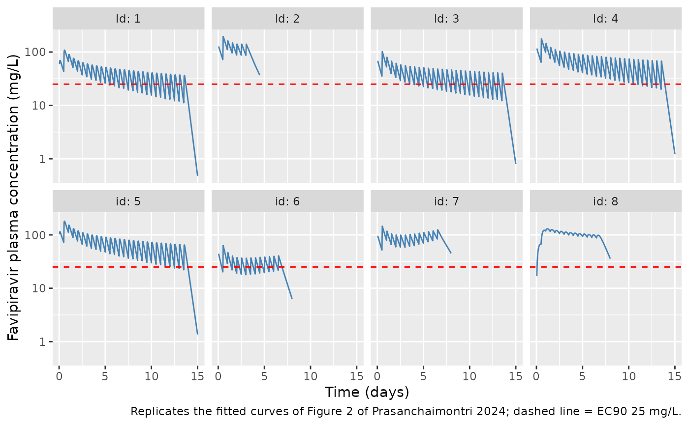
The Results report that measured Cmin and Cmax ranged from 12.1 to 132.2 mg/L and 14.5 to 201.2 mg/L across patients and days. The fitted curves span a comparable range during dosing.
# Restrict to the dosing period: from the second dose to each patient's last dose.
last_dose <- tibble::tibble(id = seq_along(dose_days), last_dose = (round(dose_days * 2) - 1) * 12)
sim_ind |>
  dplyr::left_join(last_dose, by = "id") |>
  dplyr::filter(time >= 12, time <= last_dose) |>
  dplyr::summarise("Lowest fitted Cc (mg/L)" = min(Cc), "Highest fitted Cc (mg/L)" = max(Cc)) |>
knitr::kable(digits = 1)| Lowest fitted Cc (mg/L) | Highest fitted Cc (mg/L) |
|---|---|
| 11.2 | 195.9 |
Virtual cohort and Figure 3
Figure 3 of the paper shows the 90 % prediction interval of 1000 simulated profiles drawn from the Table 1 parameters. Panel A uses the Thai regimen (1800/800 mg twice daily) and panel D the 1600/600 mg regimen used in the Turkish study. Here 200 virtual patients per regimen are simulated over 15 days, with 14 days of twice-daily dosing.
rxode2::rxSetSeed(20241107)
n_per_arm <- 200
regimens <- tibble::tibble(
  regimen = c("1800/800 mg BID", "1600/600 mg BID"),
  loading = c(1800, 1600),
  maintenance = c(800, 600)
)
obs_times <- seq(0, 360, by = 1)
ev_pop <- dplyr::bind_rows(lapply(seq_len(nrow(regimens)), function(r) {
  ids <- (r - 1) * n_per_arm + seq_len(n_per_arm)
  dose_time <- seq(0, 324, by = 12)
  doses <- tidyr::expand_grid(id = ids, time = dose_time) |>
    dplyr::mutate(evid = 1L, cmt = "depot",
                  amt = ifelse(time < 24, regimens$loading[r], regimens$maintenance[r]))
  obs <- tidyr::expand_grid(id = ids, time = obs_times) |>
    dplyr::mutate(evid = 0L, cmt = "central", amt = 0)
  dplyr::bind_rows(doses, obs) |>
    dplyr::mutate(regimen = regimens$regimen[r])
})) |>
  dplyr::arrange(id, time, dplyr::desc(evid))

sim_pop <- rxode2::rxSolve(mod, events = ev_pop, keep = "regimen",
                           returnType = "data.frame")
#> ℹ parameter labels from comments will be replaced by 'label()'
band <- sim_pop |>
  dplyr::group_by(regimen, time) |>
  dplyr::summarise(
    Q05 = quantile(Cc, 0.05), Q50 = median(Cc), Q95 = quantile(Cc, 0.95),
    .groups = "drop"
  )

ggplot(dplyr::filter(band, time > 0), aes(time / 24)) +
  geom_ribbon(aes(ymin = pmax(Q05, 0.05), ymax = Q95), fill = "lightblue", alpha = 0.6) +
  geom_line(aes(y = Q50), colour = "steelblue") +
  geom_hline(yintercept = 25, colour = "red") +
  facet_wrap(~regimen) +
  scale_y_log10(limits = c(0.05, 500)) +
  labs(x = "Time (days)", y = "Favipiravir plasma concentration (mg/L)",
       caption = paste("Replicates Figure 3A (1800/800 mg) and 3D (1600/600 mg) of",
                       "Prasanchaimontri 2024: median and 90% prediction interval."))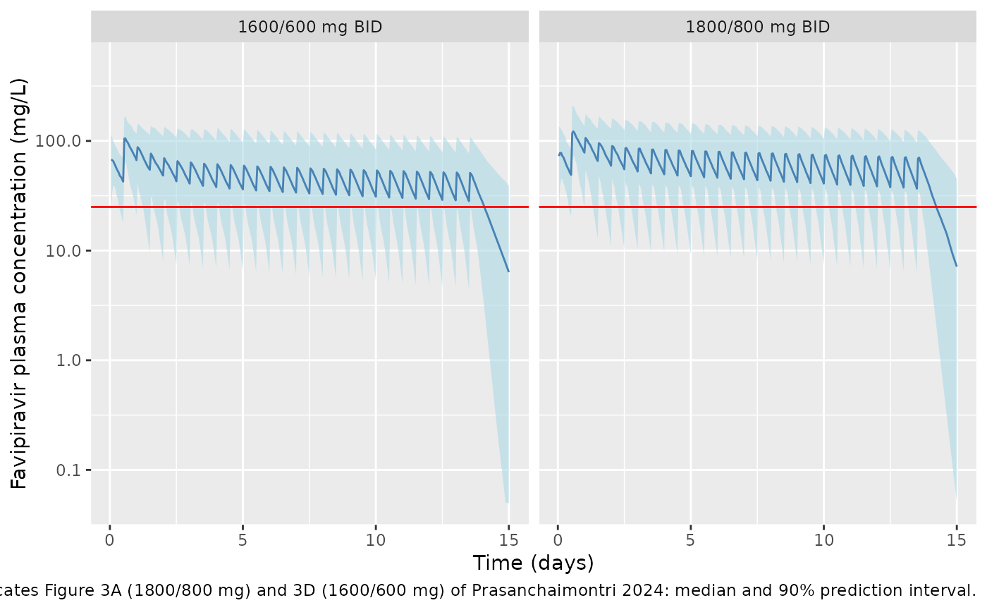
Read from Figure 3A, the published median is about 36 mg/L at the day-13 trough and about 6.5 mg/L at day 15, 36 h after the last dose. The simulated medians are compared below.
fig3a <- band |>
  dplyr::filter(regimen == "1800/800 mg BID", time %in% c(312, 360)) |>
  dplyr::mutate(
    timepoint = ifelse(time == 312, "Day 13 trough (312 h)", "Day 15 (360 h)"),
    published_median = ifelse(time == 312, 36, 6.5)
  ) |>
  dplyr::select(timepoint, published_median, simulated_median = Q50,
                simulated_Q05 = Q05, simulated_Q95 = Q95)
fig3a |>
  dplyr::rename(
    "Time point" = timepoint,
    "Figure 3A median (mg/L, read from plot)" = published_median,
    "Simulated median (mg/L)" = simulated_median,
    "Simulated 5th percentile" = simulated_Q05,
    "Simulated 95th percentile" = simulated_Q95
  ) |>
knitr::kable(digits = 1)| Time point | Figure 3A median (mg/L, read from plot) | Simulated median (mg/L) | Simulated 5th percentile | Simulated 95th percentile |
|---|---|---|---|---|
| Day 13 trough (312 h) | 36.0 | 37.5 | 6.5 | 98.3 |
| Day 15 (360 h) | 6.5 | 7.1 | 0.1 | 44.9 |
# Medians only: the tails of a 200-subject cohort are not reproducible across
# rxode2 builds, and the published values are read from a plot.
stopifnot(
  abs(fig3a$simulated_median[1] / 36 - 1) < 0.25,
  abs(fig3a$simulated_median[2] / 6.5 - 1) < 0.5
)
Distribution of the daily change in CL/F
Table 1 summarises the daily change in CL/F only on the arithmetic scale, and three of the eight individual values are negative, so the paper does not say how it was distributed in the simulations. The chunk below draws one set of CL/F, V/F and ka values in base R and pairs it with three readings of the daily change: a normal distribution with the Table 1 SD, a log-normal distribution moment-matched to the Table 1 mean and variance, and the fixed mean that the packaged model uses.
set.seed(20241107)
n_alt <- 200
base_draw <- tibble::tibble(
  id = seq_len(n_alt),
  lcl = log(1.0) + rnorm(n_alt, 0, sqrt(0.3)),
  lvc = log(19.5) + rnorm(n_alt, 0, sqrt(0.1)),
  lka = log(3.4) + rnorm(n_alt, 0, sqrt(1.8))
)
slope_var <- 57.3 / 100^2 # Table 1 'Variance' of the daily % change, as a fraction
ln_sigma2 <- log(1 + slope_var / 0.024^2)
slope_draws <- list(
  "Normal, SD 7.6 %" = rnorm(n_alt, 0.024, sqrt(slope_var)),
  "Log-normal, moment-matched" = exp(rnorm(n_alt, log(0.024) - ln_sigma2 / 2, sqrt(ln_sigma2))),
  "Fixed 2.4 % (packaged)" = rep(0.024, n_alt)
)
ev_alt <- ev_pop |>
  dplyr::filter(regimen == "1800/800 mg BID") |>
  dplyr::select(-regimen)
alt <- dplyr::bind_rows(lapply(names(slope_draws), function(nm) {
  p <- dplyr::mutate(base_draw, cl_time_slope = slope_draws[[nm]])
  rxode2::rxSolve(mod_typical, events = ev_alt, params = p, returnType = "data.frame") |>
    dplyr::filter(time %in% c(312, 360)) |>
    dplyr::mutate(reading = nm)
}))
#> ℹ omega/sigma items treated as zero: 'etalka', 'etalcl', 'etalvc'
#> Warning: multi-subject simulation without without 'omega'
#> ℹ omega/sigma items treated as zero: 'etalka', 'etalcl', 'etalvc'
#> Warning: multi-subject simulation without without 'omega'
#> ℹ omega/sigma items treated as zero: 'etalka', 'etalcl', 'etalvc'
#> Warning: multi-subject simulation without without 'omega'
alt_summary <- alt |>
  dplyr::group_by(reading, time) |>
  dplyr::summarise(median = median(Cc), q95 = quantile(Cc, 0.95), .groups = "drop")
alt_summary |>
  dplyr::rename("Reading" = reading, "Time (h)" = time,
                "Median Cc (mg/L)" = median, "95th percentile Cc (mg/L)" = q95) |>
knitr::kable(digits = 1, caption = "Figure 3A at the day-13 trough (312 h) and day 15 (360 h) under three readings of the daily change in CL/F.")| Reading | Time (h) | Median Cc (mg/L) | 95th percentile Cc (mg/L) |
|---|---|---|---|
| Fixed 2.4 % (packaged) | 312 | 39.2 | 120.1 |
| Fixed 2.4 % (packaged) | 360 | 7.7 | 56.8 |
| Log-normal, moment-matched | 312 | 43.6 | 124.1 |
| Log-normal, moment-matched | 360 | 9.5 | 70.8 |
| Normal, SD 7.6 % | 312 | 40.9 | 1216.9 |
| Normal, SD 7.6 % | 360 | 9.0 | 2276.1 |
# Share of subjects whose CL/F reaches zero or below by day 14 under the
# normal reading: 1 + slope * 13 <= 0.
mean(1 + slope_draws[["Normal, SD 7.6 %"]] * 13 <= 0)
#> [1] 0.1
Figure 3A shows a day-15 upper bound of about 50 mg/L. Under the normal reading, the subjects whose CL/F falls to zero accumulate drug, and the 95th percentile climbs far above that. The packaged fixed-mean reading reproduces the published median line most closely.
q95_d15 <- setNames(
  alt_summary$q95[alt_summary$time == 360],
  alt_summary$reading[alt_summary$time == 360]
)
# The normal reading's upper tail is driven by CL/F reaching zero; it sits
# several-fold above the fixed-mean reading in any cohort of this size.
stopifnot(q95_d15[["Normal, SD 7.6 %"]] > 3 * q95_d15[["Fixed 2.4 % (packaged)"]])
PKNCA validation
The paper does not report NCA parameters. PKNCA is run on the simulated 1800/800 mg and 1600/600 mg cohorts over the first dosing interval (0-12 h, after the 1800 or 1600 mg loading dose) and over a day-13 interval (300-312 h) to show the decline in exposure as CL/F rises by 2.4 % per day.
sim_nca <- sim_pop |>
  dplyr::filter(!is.na(Cc)) |>
  dplyr::select(id, time, Cc, regimen)
sim_nca <- dplyr::bind_rows(
  sim_nca,
  sim_nca |> dplyr::distinct(id, regimen) |> dplyr::mutate(time = 0, Cc = 0)
) |>
  dplyr::distinct(id, regimen, time, .keep_all = TRUE) |>
  dplyr::arrange(id, regimen, time)

dose_df <- ev_pop |>
  dplyr::filter(evid == 1) |>
  dplyr::select(id, time, amt, regimen)

conc_obj <- PKNCA::PKNCAconc(sim_nca, Cc ~ time | regimen + id)
dose_obj <- PKNCA::PKNCAdose(dose_df, amt ~ time | regimen + id)
intervals <- data.frame(
  start = c(0, 300), end = c(12, 312),
  cmax = TRUE, cmin = TRUE, tmax = TRUE, auclast = TRUE
)
nca_res <- PKNCA::pk.nca(PKNCA::PKNCAdata(conc_obj, dose_obj, intervals = intervals))

nca_summary <- as.data.frame(nca_res$result) |>
  dplyr::filter(PPTESTCD %in% c("cmax", "cmin", "auclast")) |>
  dplyr::group_by(regimen, start, end, PPTESTCD) |>
  dplyr::summarise(median = median(PPORRES), .groups = "drop") |>
  tidyr::pivot_wider(names_from = PPTESTCD, values_from = median)

nca_summary |>
  dplyr::rename(
    "Regimen" = regimen, "Start (h)" = start, "End (h)" = end,
    "Median Cmax (mg/L)" = cmax, "Median Cmin (mg/L)" = cmin,
    "Median AUC0-12 (mg*h/L)" = auclast
  ) |>
knitr::kable(digits = 1, caption = "Simulated NCA by regimen and dosing interval.")| Regimen | Start (h) | End (h) | Median AUC0-12 (mg*h/L) | Median Cmax (mg/L) | Median Cmin (mg/L) |
|---|---|---|---|---|---|
| 1600/600 mg BID | 0 | 12 | 640.3 | 70.4 | 0.0 |
| 1600/600 mg BID | 300 | 312 | 477.5 | 53.7 | 28.7 |
| 1800/800 mg BID | 0 | 12 | 757.2 | 83.8 | 0.0 |
| 1800/800 mg BID | 300 | 312 | 632.0 | 74.9 | 37.5 |
Over a 12-hour interval at steady state, AUC equals dose / (CL/F). The day-13 median AUC for the 1800/800 mg regimen should therefore be near 800 / (1.0 * (1 + 0.024 * 12)) = 621 mg*h/L, less a few percent because steady state is approached under a clearance that keeps rising.
Assumptions and deviations
-
Two-stage summary as a population model. The paper
estimated no population parameters. Typical values are the Table 1
geometric means and the between-subject variances the variances of the
log-transformed individual estimates, which is how the Methods describe
the population simulations (“assuming log-normal distributions”). All
are wrapped in
fixed()to show that none was estimated as a population parameter. -
No between-subject variability on the daily change in
CL/F. Table 1 gives the daily change only as an arithmetic mean
(2.4 %) and variance (57.3, SD 7.6 %); no log-scale summary is possible
because three of the eight individual values are negative. The section
“Distribution of the daily change in CL/F” compares three readings
against Figure 3A. A normal distribution with SD 7.6 % sends CL/F to
zero or below by day 14 in about one subject in ten and pushes the 95th
percentile far above the published interval, so the authors cannot have
simulated it. A log-normal distribution moment-matched to the arithmetic
mean and variance raises the day-15 median above the published line. A
fixed 2.4 % per day reproduces the published median (about 36 mg/L at
the day-13 trough and 6.5 mg/L at day 15), so that reading is packaged.
Users who want the observed spread can add an additive eta on
cl_time_slopewith variance 0.00573, keeping in mind that it allows CL/F to become non-positive in long simulations. -
Dosing-day index. The equation’s day number
nis taken as the day counted from the first dose at time 0 (floor(t / 24) + 1), so CL/F steps up once every 24 h. The paper does not say whether the change continues after dosing stops; the model continues it, which affects only the washout tail. -
Residual error. The fits used 1/predicted^2
weighting (proportional error) but no magnitude was reported, so
propSdis fixed at 0. - ka. The individual ka estimates are imprecise (RSE up to 14982 %), which drives the large log-variance (1.8). The abstract quotes a mean ka of “6.1 h”; Table 1 gives an arithmetic mean of 6.0 1/h and the Results text 6.1 1/h. The geometric mean (3.4 1/h) is packaged.
- Metabolite. T-705M1 was measured but not modelled.
- No erratum was found for this article (Europe PMC search, 2026-10-31).