Vildagliptin plasma, muscle and liver exposure in diabetic rats and its human projection (Dias 2026)
Source:vignettes/articles/Dias_2026_vildagliptin.Rmd
Dias_2026_vildagliptin.Rmd
mod_rat <- rxode2::rxode2(readModelDb("Dias_2026_vildagliptin_rat"))
#> ℹ parameter labels from comments will be replaced by 'label()'
mod_human <- rxode2::rxode2(readModelDb("Dias_2026_vildagliptin_human"))
Model and source
- Citation: Dias BB, Olivo LB, de Araujo BV. Preclinical Modeling and Simulation to Explore the Tissue/Plasma Exposure and Pharmacodynamic Effect of Vildagliptin in Diabetes Treatment. CPT Pharmacometrics Syst Pharmacol. 2026;15(2):e70165. doi:10.1002/psp4.70165. PMCID: PMC12896384. Parameter estimates: Table 1. Structural ODEs: Equations 4-7 and Figure 2. Group sizes: Supporting Information Table S1.
- Rat model: Preclinical (rat, male Wistar). Four-compartment population PK model for intravenous vildagliptin in healthy rats and in rats with alloxan-induced diabetes, fit jointly to plasma and to unbound skeletal muscle and liver interstitial concentrations measured by microdialysis (Dias 2026). The ODE states carry UNBOUND drug amounts per kg body weight: a central (plasma) compartment with linear elimination, a peripheral compartment, and muscle and liver compartments each linked to central by separate influx and efflux clearances. Diabetes has its own central-peripheral clearance Q1 and liver efflux clearance. Total plasma is unbound plasma divided by the unbound fraction 0.91. IIV on CL, Q1, the muscle and liver volumes and the liver efflux clearance; log-additive residual error per matrix.
- Human projection: Allometric human projection of the Dias 2026 rat vildagliptin model for patients with type 2 diabetes, with an Imax model of DPP-4 inhibition by unbound plasma, skeletal-muscle and liver concentrations. Four-compartment disposition (central, peripheral, muscle and liver, the tissues linked to central by separate influx and efflux clearances) whose clearances and volumes are the diabetic-rat per-kg estimates scaled by Equation 2 (exponent 0.75 for clearances, 1 for volumes; rat reference 0.35 kg), with oral absorption through two sequential first-order steps and bioavailability 77.2% taken from Landersdorfer 2012. Typical-value simulation model: no IIV and no residual error.
- Article: https://doi.org/10.1002/psp4.70165 (PMC12896384, open access). Supporting Information: bioanalytical method, Table S1 (animals and observations) and Table S2 (human parameters).
Dias et al. gave vildagliptin 50 mg/kg as an intravenous bolus to healthy male Wistar rats and to rats with alloxan-induced diabetes. They measured total plasma concentrations and unbound concentrations in skeletal muscle and liver by microdialysis. The final model (Figure 2 of the paper) has four compartments, all carrying unbound drug:
- central (plasma), with linear clearance;
- a peripheral compartment;
- muscle and liver, each linked to central by its own influx clearance (Qin) and efflux clearance (Qout).
Diabetes changes two parameters: it raises the central-peripheral clearance Q1 about eightfold and lowers the liver efflux clearance about elevenfold, so unbound liver concentrations are much higher in diabetic rats.
The paper then scales the rat parameters to a patient with type 2
diabetes by allometry (Equation 2), adds the oral absorption of
Landersdorfer 2012, and converts the predicted unbound concentrations to
DPP-4 inhibition with an Imax model (Equation 3). The two parts are
packaged as two models: Dias_2026_vildagliptin_rat (the
fitted model) and Dias_2026_vildagliptin_human (the
projection).
Population
| Field | Value |
|---|---|
| Species | rat (Wistar, male) |
| Animals | 37 |
| Weight | 250-350 g |
| Female | 0% |
| Groups | Healthy rats and rats with alloxan-induced diabetes (blood glucose > 300 mg/dL; studied 4 weeks after induction). |
| Dose | Single 50 mg/kg intravenous bolus. |
| Region | Brazil (Federal University of Rio Grande do Sul, Porto Alegre) |
Each animal contributed one matrix (Supporting Information Table S1):
plasma from 7 healthy and 5 diabetic rats, liver microdialysate from 6
and 6, and muscle microdialysate from 7 and 6, for 254 observations in
all. Diabetes is encoded with DIS_DIAB (1 = diabetic). The
rat parameters are per kg body weight and the dose is entered in
mg/kg.
The human model was not fit to any human data. It describes a typical
91 kg patient with type 2 diabetes (WT = 91; see the
assumptions below).
Source trace
| Model element | Value in file | Source location |
|---|---|---|
d/dt(central) |
Q1/V2 A2 + Qout,m/V3 A3 + Qout,l/V4 A4 - (CL + Q1 + Qin,m + Qin,l)/V1 A1 | Equation 4 |
d/dt(peripheral1) |
Q1/V1 A1 - Q1/V2 A2 | Equation 5 |
d/dt(muscle) |
Qin,m/V1 A1 - Qout,m/V3 A3 | Equation 6 |
d/dt(liver) |
Qin,l/V1 A1 - Qout,l/V4 A4 | Equation 7 |
Cu, Cmuscle, Cliver
|
A1/V1, A3/V3, A4/V4 | Figure 2 |
Cc (rat, total plasma) |
Cu / 0.91 | Methods ‘Model Building’ (9% protein binding) |
| Diabetes | separate Q1 and Qout,liver, one eta each | Methods ‘Covariate Analysis’; Results; Table 1 |
lcl |
log(2.72) L/h/kg | Table 1, CL |
lvc |
log(1.11) L/kg | Table 1, V1 |
lq, lq_diabetic
|
log(0.338), log(2.61) L/h/kg | Table 1, Q1,healthy and Q1,diabetic |
lvp |
log(1.85) L/kg | Table 1, V2 |
lclin_muscle, lclef_muscle
|
log(2.09), log(14.3) L/h/kg | Table 1, Qin,muscle and Qout,muscle |
lv_muscle |
log(2.55) L/kg | Table 1, V3 |
lclin_liver |
log(2.5) L/h/kg | Table 1, Qin,liver |
lclef_liver, lclef_liver_diabetic
|
log(218), log(19.7) L/h/kg | Table 1, Qout,liver,healthy and Qout,liver,diabetic |
lv_liver |
log(0.856) L/kg | Table 1, V4 |
fu |
0.91 (fixed) | Methods ‘Model Building’ |
etalcl, etalq, etalv_muscle,
etalclef_liver, etalv_liver
|
0.192^2, 0.654^2, 0.766^2, 0.720^2, 1.814^2 | Table 1, IIV column; footnote: CV% = omega x 100 |
expSd, expSd_Cmuscle,
expSd_Cliver
|
0.213, 0.217, 0.159 | Table 1, residual error rows |
| Human scaling | per-kg value x 0.35 x (WT/0.35)^b | Equation 2; b from Methods ‘Allometry’; weights from Table S2 (see below) |
e_wt_cl, e_wt_vc
|
0.75, 1 (fixed) | Methods ‘Allometry’ |
Human lq, lclef_liver
|
diabetic values 2.61, 19.7 L/h/kg | Table S2 (‘PK parameters for diabetic patients’) |
lktr, lka
|
log(1.26), log(1.05) 1/h (fixed) | Methods ‘Allometry’ (Ka1, Ka2 of Landersdorfer 2012) |
lfdepot |
log(0.772) (fixed) | Methods ‘Allometry’ (Fabs) |
limax |
log(100) % (fixed) | Not printed; Figure 5 |
lic50 |
log(1.35) ng/mL (fixed) | Figure 5 caption; Methods (4.5 nmol/L) |
inh_plasma, inh_muscle,
inh_liver
|
Imax Cu / (Cu + IC50) | Equation 3 |
Dimensional check: in the rat model doses are mg/kg, volumes L/kg and clearances L/h/kg, so every term of Equations 4-7 is in mg/h/kg and every concentration is in mg/L, the unit of Figures 1 and 4. In the human model the doses are mg, volumes L and clearances L/h, and the concentrations are multiplied by 1000 to give ng/mL, the unit of Figure 5.
Rat: single 50 mg/kg intravenous bolus
There are 100 virtual rats per group. Every model variable is
returned at the observation rows, so the unbound plasma
(Cu) and the total plasma (Cc) are both
available.
n_per_group <- 100L
rat_times <- sort(unique(c(seq(0, 6, by = 1 / 60), 0.083, 0.166, 0.2)))

rat_events <- function(diab, id_offset) {
  ev <- rxode2::et(amt = 50, cmt = "central") |>
    rxode2::et(rat_times, cmt = "central") |>
    as.data.frame()
  # Three ~ endpoints: observation rows carry dvid = 1; Cc, Cu, Cmuscle and
  # Cliver are all returned as columns.
  ev$dvid <- ifelse(ev$evid == 0, 1L, NA_integer_)
  tidyr::expand_grid(id = id_offset + seq_len(n_per_group), ev) |>
    mutate(DIS_DIAB = diab, group = ifelse(diab == 1L, "Diabetic", "Healthy"))
}

rat_ev <- bind_rows(rat_events(0L, 0L), rat_events(1L, n_per_group)) |>
  arrange(id, time, desc(evid))

rxode2::rxSetSeed(2026)
rat_sim <- rxode2::rxSolve(mod_rat, rat_ev, keep = "group") |>
  as.data.frame()

# One typical rat per group, solved one at a time: omega = NA drops the
# between-animal variability.
rat_typ <- bind_rows(lapply(c(1L, n_per_group + 1L), function(i) {
  rxode2::rxSolve(mod_rat, rat_ev |> filter(id == i), keep = "group", omega = NA) |>
    as.data.frame()
}))
rat_typ |>
  filter(time >= 0.083) |>
  select(group, time, `Total plasma` = Cc, `Free muscle` = Cmuscle, `Free liver` = Cliver) |>
  pivot_longer(-c(group, time), names_to = "matrix", values_to = "conc") |>
  ggplot(aes(time, conc, linetype = matrix, colour = matrix)) +
  geom_line(linewidth = 0.8) +
  facet_wrap(~group) +
  scale_y_log10() +
  labs(x = "Time after dose (h)", y = "Vildagliptin (mg/L)", colour = NULL, linetype = NULL) +
  theme_bw() +
  theme(legend.position = "top")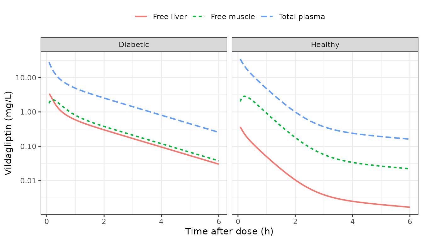
Typical-value profiles after 50 mg/kg intravenous vildagliptin (compare with the observed means of Figure 1).
The muscle compartment equilibrates with unbound plasma at Qout,muscle / V3 (about 5.6 per hour) and settles at Qin / Qout = 0.15 of it. The liver equilibrates far faster in healthy rats (Qout,liver / V4 = 255 per hour), at 0.011 of unbound plasma; in diabetic rats Qout,liver falls to 19.7 L/h/kg and the liver settles at 0.13 of unbound plasma. This reproduces the observation behind the paper’s main conclusion: diabetes leaves plasma and muscle exposure almost unchanged but raises the unbound liver exposure about elevenfold (Figure 1).
trapz <- function(t, y) sum(diff(t) * (head(y, -1) + tail(y, -1)) / 2)
typ_auc <- rat_typ |>
  group_by(group) |>
  summarise(plasma = trapz(time, Cc), muscle = trapz(time, Cmuscle),
            liver = trapz(time, Cliver), .groups = "drop")
auc_ratio <- unlist(typ_auc[typ_auc$group == "Diabetic", -1]) /
  unlist(typ_auc[typ_auc$group == "Healthy", -1])
round(auc_ratio, 2)
#> plasma muscle  liver
#>   1.03   1.03  11.50
stopifnot(
  # Typical values: deterministic. Diabetes leaves plasma and muscle AUC0-6
  # within a few percent and multiplies liver AUC0-6 about elevenfold.
  abs(auc_ratio[["plasma"]] - 1) < 0.1,
  abs(auc_ratio[["muscle"]] - 1) < 0.1,
  auc_ratio[["liver"]] > 8
)
At single time points the diabetic muscle concentration can still differ by up to twofold, because the faster central-peripheral exchange in diabetic rats changes the shape of the plasma curve; the total exposure does not.
Figure 1: observed means
Figure 1 of the paper shows the mean of the observations at each sampling time. The maintainers read the means off the published figure for total plasma (healthy and diabetic), healthy muscle and the liver (healthy and diabetic). Diabetic muscle is hidden under the diabetic liver series in the figure and is not compared. The microdialysis samples were 40-minute collections and the paper fit the average concentration over each collection interval, so the simulated tissue concentrations are averaged over the 40 minutes before each nominal time. The observed means can only include quantifiable samples: the healthy-liver means level off at about 0.034 mg/L and stop after 4 h, right at the tissue limit of quantification (10 ng/mL in dialysate, about 0.032 mg/L after the recovery correction). The comparison therefore uses the arithmetic mean of the simulated values above the same limits, and also shows what fraction of the virtual cohort is above them.
fig1 <- tibble::tribble(
  ~group,     ~matrix,        ~time, ~obs_mean,
  "Healthy",  "Total plasma", 0.083, 38,
  "Healthy",  "Total plasma", 0.5,   14,
  "Healthy",  "Total plasma", 1,     5.8,
  "Healthy",  "Total plasma", 2,     2.2,
  "Healthy",  "Total plasma", 4,     0.5,
  "Healthy",  "Total plasma", 6,     0.33,
  "Diabetic", "Total plasma", 0.083, 28,
  "Diabetic", "Total plasma", 0.5,   12,
  "Diabetic", "Total plasma", 1,     3.5,
  "Diabetic", "Total plasma", 2,     1.5,
  "Diabetic", "Total plasma", 4,     0.6,
  "Diabetic", "Total plasma", 6,     0.22,
  "Healthy",  "Free muscle",  0.667, 2.6,
  "Healthy",  "Free muscle",  1.333, 1.2,
  "Healthy",  "Free muscle",  2,     0.65,
  "Healthy",  "Free muscle",  2.667, 0.25,
  "Healthy",  "Free muscle",  3.333, 0.13,
  "Healthy",  "Free muscle",  4,     0.065,
  "Healthy",  "Free muscle",  6,     0.025,
  "Healthy",  "Free liver",   0.667, 0.28,
  "Healthy",  "Free liver",   1.333, 0.10,
  "Healthy",  "Free liver",   2,     0.075,
  "Healthy",  "Free liver",   2.667, 0.045,
  "Healthy",  "Free liver",   3.333, 0.034,
  "Healthy",  "Free liver",   4,     0.034,
  "Diabetic", "Free liver",   0.667, 2.4,
  "Diabetic", "Free liver",   1.333, 1.0,
  "Diabetic", "Free liver",   2,     0.75,
  "Diabetic", "Free liver",   2.667, 0.5,
  "Diabetic", "Free liver",   3.333, 0.33,
  "Diabetic", "Free liver",   4,     0.2,
  "Diabetic", "Free liver",   6,     0.05
)

# Limits of quantification (Supporting Information): 50 ng/mL in plasma;
# 10 ng/mL in dialysate, i.e. 10 / 0.312 = 32 ng/mL in tissue after the
# 31.2% in vivo recovery correction.
loq_plasma <- 0.05 # mg/L
loq_tissue <- 0.010 / 0.312 # mg/L

cohort_values_at <- function(grp, mtx, t) {
  d <- rat_sim |> filter(group == grp)
  if (mtx == "Total plasma") {
    return(d$Cc[abs(d$time - t) < 1e-3])
  }
  col <- if (mtx == "Free muscle") "Cmuscle" else "Cliver"
  # Average over the 40-minute collection window per animal.
  d |>
    filter(time > t - 40 / 60 + 1e-6, time <= t + 1e-6) |>
    group_by(id) |>
    summarise(v = mean(.data[[col]]), .groups = "drop") |>
    pull(v)
}

fig1_cmp <- fig1 |>
  rowwise() |>
  mutate(
    loq = ifelse(matrix == "Total plasma", loq_plasma, loq_tissue),
    vals = list(cohort_values_at(group, matrix, time)),
    pct_quantifiable = 100 * mean(vals >= loq),
    # Figure 1 averages the quantifiable samples only, so the simulated
    # mean does the same.
    sim_mean = mean(vals[vals >= loq])
  ) |>
  ungroup() |>
  select(-vals) |>
  mutate(ratio = sim_mean / obs_mean)

fig1_cmp |>
  select(-loq) |>
  mutate(across(c(obs_mean, sim_mean), \(x) signif(x, 3)), ratio = round(ratio, 2),
         pct_quantifiable = round(pct_quantifiable)) |>
  rename(Group = group, Matrix = matrix, `Time (h)` = time,
         `Figure 1 mean (mg/L)` = obs_mean,
         `Simulated >= LOQ (%)` = pct_quantifiable,
         `Simulated mean of quantifiable (mg/L)` = sim_mean,
         `Simulated / observed` = ratio) |>
knitr::kable()| Group | Matrix | Time (h) | Figure 1 mean (mg/L) | Simulated >= LOQ (%) | Simulated mean of quantifiable (mg/L) | Simulated / observed |
|---|---|---|---|---|---|---|
| Healthy | Total plasma | 0.083 | 38.000 | 100 | 33.8000 | 0.89 |
| Healthy | Total plasma | 0.500 | 14.000 | 100 | 11.0000 | 0.79 |
| Healthy | Total plasma | 1.000 | 5.800 | 100 | 4.6600 | 0.80 |
| Healthy | Total plasma | 2.000 | 2.200 | 100 | 1.3200 | 0.60 |
| Healthy | Total plasma | 4.000 | 0.500 | 95 | 0.3830 | 0.77 |
| Healthy | Total plasma | 6.000 | 0.330 | 86 | 0.2260 | 0.68 |
| Diabetic | Total plasma | 0.083 | 28.000 | 100 | 27.6000 | 0.99 |
| Diabetic | Total plasma | 0.500 | 12.000 | 100 | 8.0700 | 0.67 |
| Diabetic | Total plasma | 1.000 | 3.500 | 100 | 4.7500 | 1.36 |
| Diabetic | Total plasma | 2.000 | 1.500 | 100 | 2.4900 | 1.66 |
| Diabetic | Total plasma | 4.000 | 0.600 | 100 | 0.8960 | 1.49 |
| Diabetic | Total plasma | 6.000 | 0.220 | 99 | 0.3580 | 1.63 |
| Healthy | Free muscle | 0.667 | 2.600 | 100 | 2.0700 | 0.79 |
| Healthy | Free muscle | 1.333 | 1.200 | 100 | 0.9530 | 0.79 |
| Healthy | Free muscle | 2.000 | 0.650 | 100 | 0.3750 | 0.58 |
| Healthy | Free muscle | 2.667 | 0.250 | 95 | 0.1910 | 0.76 |
| Healthy | Free muscle | 3.333 | 0.130 | 76 | 0.1340 | 1.03 |
| Healthy | Free muscle | 4.000 | 0.065 | 58 | 0.1090 | 1.68 |
| Healthy | Free muscle | 6.000 | 0.025 | 41 | 0.0619 | 2.48 |
| Healthy | Free liver | 0.667 | 0.280 | 99 | 0.3030 | 1.08 |
| Healthy | Free liver | 1.333 | 0.100 | 65 | 0.1210 | 1.21 |
| Healthy | Free liver | 2.000 | 0.075 | 27 | 0.0886 | 1.18 |
| Healthy | Free liver | 2.667 | 0.045 | 13 | 0.0725 | 1.61 |
| Healthy | Free liver | 3.333 | 0.034 | 8 | 0.0593 | 1.75 |
| Healthy | Free liver | 4.000 | 0.034 | 5 | 0.0495 | 1.46 |
| Diabetic | Free liver | 0.667 | 2.400 | 100 | 1.7100 | 0.71 |
| Diabetic | Free liver | 1.333 | 1.000 | 100 | 0.7000 | 0.70 |
| Diabetic | Free liver | 2.000 | 0.750 | 100 | 0.4380 | 0.58 |
| Diabetic | Free liver | 2.667 | 0.500 | 99 | 0.3070 | 0.61 |
| Diabetic | Free liver | 3.333 | 0.330 | 97 | 0.2260 | 0.68 |
| Diabetic | Free liver | 4.000 | 0.200 | 90 | 0.1740 | 0.87 |
| Diabetic | Free liver | 6.000 | 0.050 | 57 | 0.1030 | 2.06 |
fig1_summary <- fig1_cmp |>
  group_by(group, matrix) |>
  summarise(median_ratio = median(ratio), .groups = "drop")
knitr::kable(fig1_summary, digits = 2)| group | matrix | median_ratio |
|---|---|---|
| Diabetic | Free liver | 0.70 |
| Diabetic | Total plasma | 1.43 |
| Healthy | Free liver | 1.33 |
| Healthy | Free muscle | 0.79 |
| Healthy | Total plasma | 0.78 |
stopifnot(
  # A mis-transcribed clearance or a wrong diabetes switch moves a whole
  # panel by several-fold; a factor of two absorbs read-off error and the
  # difference between a cohort mean and the paper's mean of the
  # above-LOQ observations.
  all(fig1_summary$median_ratio > 0.5),
  all(fig1_summary$median_ratio < 2)
)
The simulated means follow the observed means in every panel. In healthy liver after 2 h only a minority of the virtual rats are above the limit of quantification, which is consistent with the observed series ending at 4 h.
Figure 4: VPC percentiles
rat_sim |>
  filter(time >= 0.083) |>
  select(id, group, time, `Plasma` = Cc, `Free muscle` = Cmuscle, `Free liver` = Cliver) |>
  pivot_longer(c(Plasma, `Free muscle`, `Free liver`), names_to = "matrix", values_to = "conc") |>
  mutate(matrix = factor(matrix, levels = c("Plasma", "Free muscle", "Free liver"))) |>
  group_by(group, matrix, time) |>
  summarise(p10 = quantile(conc, 0.1), p50 = median(conc), p90 = quantile(conc, 0.9),
            .groups = "drop") |>
  ggplot(aes(time)) +
  geom_ribbon(aes(ymin = p10, ymax = p90), alpha = 0.25) +
  geom_line(aes(y = p50)) +
  facet_grid(group ~ matrix) +
  scale_y_log10() +
  labs(x = "Time after dose (h)", y = "Vildagliptin (mg/L)") +
  theme_bw()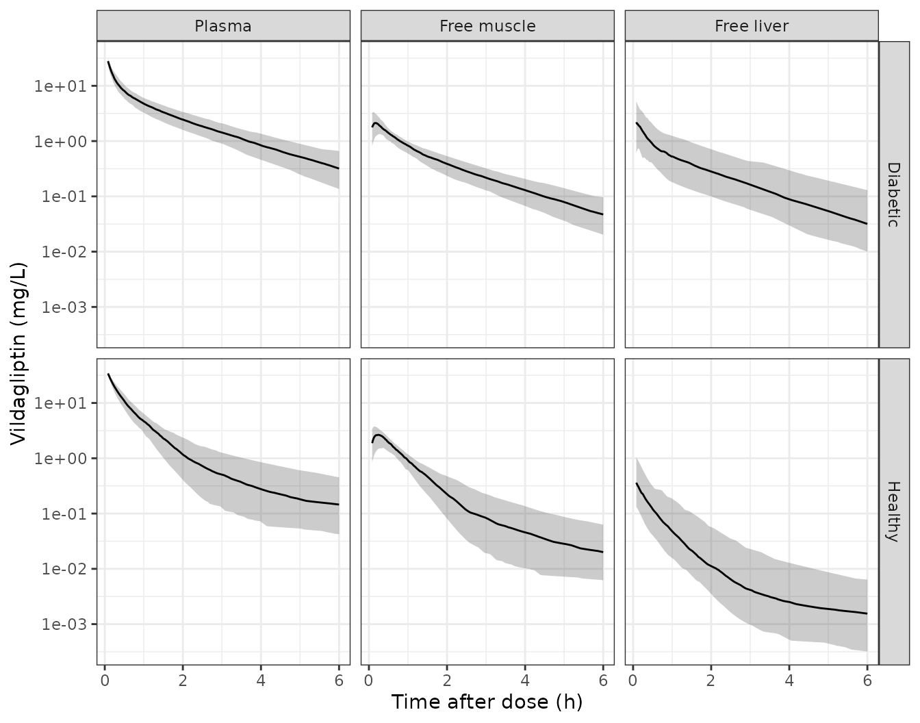
Simulated 10th, 50th and 90th percentiles by matrix and group (compare with Figure 4 of the paper).
NCA of the simulated rat profiles
The paper reports no NCA, so these values are descriptive. They summarise total plasma, unbound muscle and unbound liver exposure by group.
rat_conc <- rat_sim |>
  select(id, group, time, Cc, Cmuscle, Cliver) |>
  pivot_longer(c(Cc, Cmuscle, Cliver), names_to = "matrix", values_to = "conc") |>
  filter(!is.na(conc)) |>
  mutate(treatment = paste(group, matrix))
rat_dose <- rat_ev |>
  filter(evid == 1) |>
  distinct(id, group, time, amt) |>
  tidyr::expand_grid(matrix = c("Cc", "Cmuscle", "Cliver")) |>
  mutate(treatment = paste(group, matrix))

rat_nca <- PKNCA::pk.nca(PKNCA::PKNCAdata(
  PKNCA::PKNCAconc(rat_conc, conc ~ time | treatment + id),
  PKNCA::PKNCAdose(rat_dose, amt ~ time | treatment + id, route = "intravascular"),
  intervals = data.frame(start = 0, end = 6, cmax = TRUE, auclast = TRUE)
))
rat_nca_tab <- as.data.frame(rat_nca$result) |>
  group_by(treatment, PPTESTCD) |>
  summarise(median = signif(median(PPORRES), 3), .groups = "drop") |>
  pivot_wider(names_from = PPTESTCD, values_from = median)
rat_nca_tab |>
  rename(Group = treatment, `Cmax (mg/L)` = cmax, `AUC0-6 (h*mg/L)` = auclast) |>
knitr::kable()| Group | AUC0-6 (h*mg/L) | Cmax (mg/L) |
|---|---|---|
| Diabetic Cc | 19.300 | 49.500 |
| Diabetic Cliver | 2.000 | 2.600 |
| Diabetic Cmuscle | 2.560 | 2.160 |
| Healthy Cc | 19.400 | 49.500 |
| Healthy Cliver | 0.211 | 0.427 |
| Healthy Cmuscle | 2.560 | 2.670 |
Human projection
Table S2: the scaled parameters
Equation 2 multiplies each rat parameter by (Weight_human /
Weight_rat)^b. The paper does not state either weight. Supporting
Information Table S2 is reproduced to four significant figures by a 0.35
kg rat and a 91 kg patient (91 kg is the mean weight of the
Landersdorfer 2012 patients), and the human model computes the scaling
from the per-kg rat values at run time, so WT can be
changed.
one_patient <- rxode2::et(amt = 100, cmt = "depot") |>
  rxode2::et(c(0, 1)) |>
  as.data.frame() |>
  mutate(WT = 91)
pars <- rxode2::rxSolve(mod_human, one_patient) |> as.data.frame()

s2 <- tibble::tribble(
  ~Parameter,       ~col,          ~table_s2,
  "CL (L/h)",        "cl",          101.01,
  "V1 (L)",          "vc",          61.64,
  "Q1 (L/h)",        "q",           27.65,
  "V2 (L)",          "vp",          168.35,
  "Qin,muscle (L/h)",  "clin_muscle", 47.36,
  "Qout,muscle (L/h)", "clef_muscle", 324.07,
  "V3 (L)",          "v_muscle",    232.05,
  "Qin,liver (L/h)",   "clin_liver",  56.65,
  "Qout,liver (L/h)",  "clef_liver",  446.44,
  "V4 (L)",          "v_liver",     77.90
) |>
  mutate(model = vapply(col, \(x) pars[[x]][1], numeric(1)),
         ratio = model / table_s2)
s2 |>
  select(-col) |>
  mutate(model = round(model, 2), ratio = round(ratio, 4)) |>
  rename(`Table S2` = table_s2, `Model at WT = 91 kg` = model, `Model / Table S2` = ratio) |>
knitr::kable()| Parameter | Table S2 | Model at WT = 91 kg | Model / Table S2 |
|---|---|---|---|
| CL (L/h) | 101.01 | 61.64 | 0.6102 |
| V1 (L) | 61.64 | 101.01 | 1.6387 |
| Q1 (L/h) | 27.65 | 59.15 | 2.1392 |
| V2 (L) | 168.35 | 168.35 | 1.0000 |
| Qin,muscle (L/h) | 47.36 | 47.36 | 1.0001 |
| Qout,muscle (L/h) | 324.07 | 324.07 | 1.0000 |
| V3 (L) | 232.05 | 232.05 | 1.0000 |
| Qin,liver (L/h) | 56.65 | 56.65 | 1.0001 |
| Qout,liver (L/h) | 446.44 | 446.44 | 1.0000 |
| V4 (L) | 77.90 | 77.90 | 0.9999 |
consistent <- s2 |> filter(!col %in% c("cl", "vc", "q"))
stopifnot(
  # Deterministic arithmetic on printed values: four significant figures.
  all(abs(consistent$ratio - 1) < 1e-3),
  # Table S2 prints CL and V1 transposed.
  abs(pars$cl[1] / 61.64 - 1) < 1e-3,
  abs(pars$vc[1] / 101.01 - 1) < 1e-3
)
Seven of the ten parameters match Table S2. The other three do not:
- Table S2 gives CL = 101.01 L/h and V1 = 61.64 L. Equation 2 gives CL = 61.64 L/h and V1 = 101.01 L, the same two numbers transposed. Every other volume in Table S2 is its Table 1 value times 91, and V1 would be too if the two were swapped. The model follows Equation 2.
- Table S2 gives Q1 = 27.65 L/h. Equation 2 gives 59.15 L/h from the diabetic Q1 (2.61 L/h/kg) and 7.66 L/h from the healthy Q1 (0.338 L/h/kg); no value in Table 1 scales to 27.65. The table is titled for diabetic patients, its Qout,liver is the diabetic value, and the Discussion assumes the same diabetes effect on the intercompartmental clearances in rats and humans, so the model uses the diabetic Q1.
Figure 5: steady-state profiles
The paper simulated oral 25, 50 and 100 mg once and twice daily and plotted the fifth day (96-120 h).
regimens <- tidyr::expand_grid(dose = c(25, 50, 100), tau = c(24, 12)) |>
  mutate(regimen = paste0(dose, " mg q", tau, "h"),
         id = seq_len(n()))
ss_times <- seq(96, 120, by = 0.1)

human_ev <- bind_rows(lapply(seq_len(nrow(regimens)), function(i) {
  r <- regimens[i, ]
  rxode2::et(amt = r$dose, ii = r$tau, addl = 120 / r$tau, cmt = "depot") |>
    rxode2::et(ss_times) |>
    as.data.frame() |>
    mutate(id = r$id, regimen = r$regimen, dose = r$dose, tau = r$tau)
})) |>
  mutate(WT = 91)

human_sim <- rxode2::rxSolve(mod_human, human_ev, keep = c("regimen", "dose", "tau")) |>
  as.data.frame() |>
  filter(time >= 96)
long_human <- human_sim |>
  select(regimen, dose, tau, time, Cu, Cmuscle, Cliver, inh_plasma, inh_muscle, inh_liver) |>
  pivot_longer(c(Cu, Cmuscle, Cliver, inh_plasma, inh_muscle, inh_liver),
               names_to = "var", values_to = "value") |>
  mutate(
    quantity = ifelse(grepl("^inh", var), "DPP-4 inhibition (%)", "Unbound concentration (ng/mL)"),
    matrix = case_when(var %in% c("Cu", "inh_plasma") ~ "Plasma",
                       var %in% c("Cmuscle", "inh_muscle") ~ "Muscle",
                       TRUE ~ "Liver"),
    matrix = factor(matrix, levels = c("Plasma", "Muscle", "Liver")),
    schedule = paste0("q", tau, "h"),
    dose = factor(paste(dose, "mg"), levels = c("25 mg", "50 mg", "100 mg"))
  )

ref_lines <- tibble::tibble(
  quantity = c("Unbound concentration (ng/mL)", "DPP-4 inhibition (%)"),
  y = c(1.35, 80)
)

ggplot(long_human, aes(time, value, colour = dose)) +
  geom_line(linewidth = 0.7) +
  geom_hline(data = ref_lines, aes(yintercept = y), linetype = "dashed") +
  facet_grid(quantity ~ schedule + matrix, scales = "free_y") +
  scale_y_continuous(trans = "identity") +
  labs(x = "Time (h)", y = NULL, colour = "Dose") +
  theme_bw() +
  theme(legend.position = "bottom")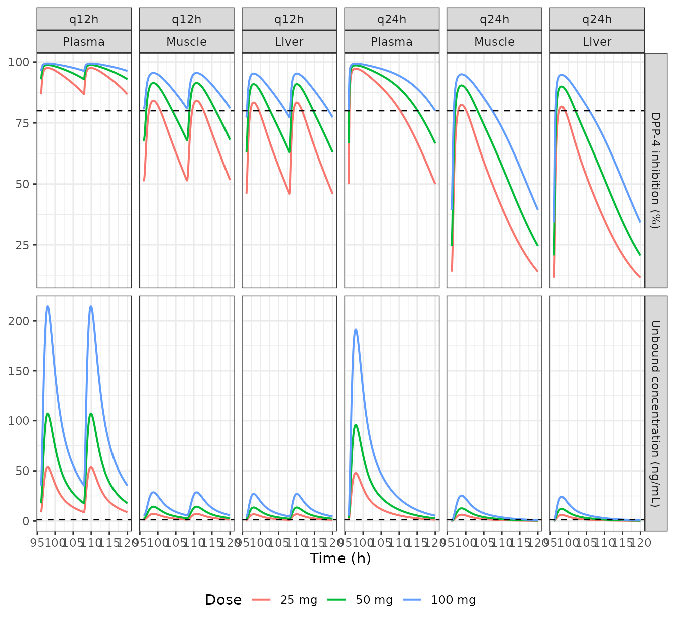
Typical steady-state unbound concentrations (top) and DPP-4 inhibition (bottom) on day 5 (replicates Figure 5; dashed lines: IC50 = 1.35 ng/mL and 80% inhibition).
long_human |>
  filter(quantity == "Unbound concentration (ng/mL)") |>
  ggplot(aes(time, value, colour = dose)) +
  geom_line(linewidth = 0.7) +
  geom_hline(yintercept = 1.35, linetype = "dashed") +
  facet_grid(schedule ~ matrix) +
  scale_y_log10() +
  labs(x = "Time (h)", y = "Unbound vildagliptin (ng/mL)", colour = "Dose") +
  theme_bw() +
  theme(legend.position = "bottom")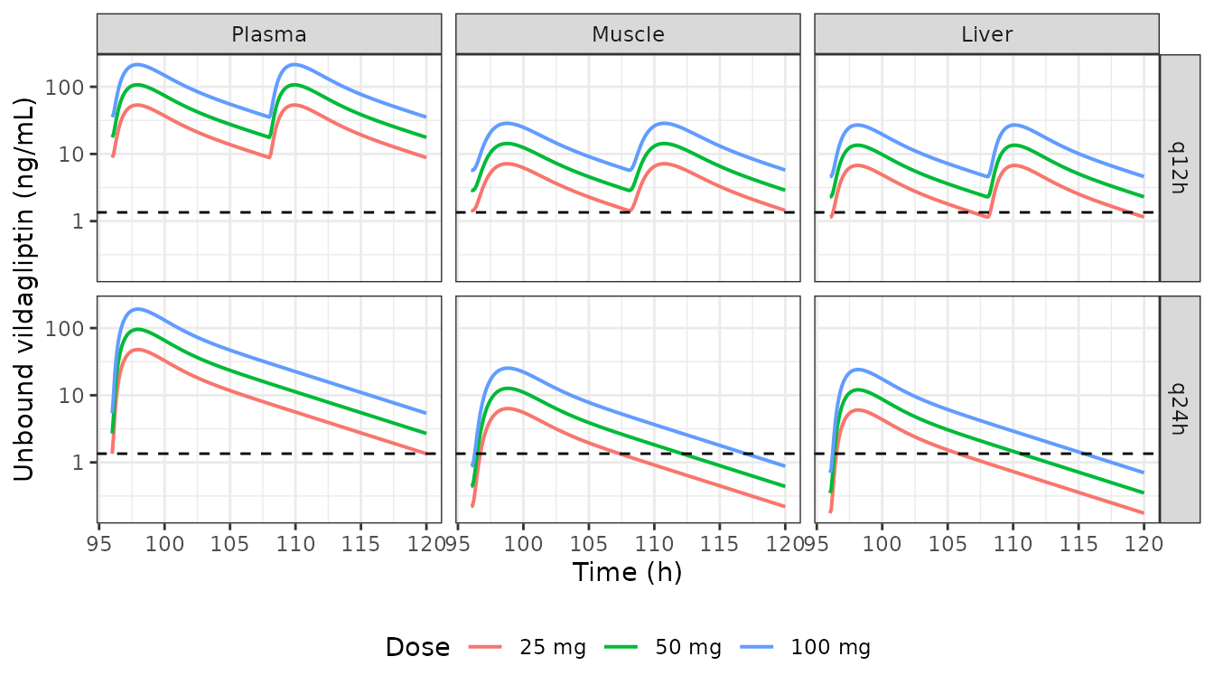
The concentration panels on a log scale, as in Figure 5.
The profiles have the shape of Figure 5: plasma peaks near 200 ng/mL after 100 mg, the tissues peak about eightfold lower, and the twice-daily regimens keep every matrix above the IC50 for longer. The Results state that after 25 and 50 mg once daily the tissue concentrations fall below the IC50 “after 16 and 20 h”; the model gives the times below.
below_ic50 <- human_sim |>
  filter(tau == 24, dose %in% c(25, 50), time > 97) |>
  select(dose, time, Cmuscle, Cliver) |>
  pivot_longer(c(Cmuscle, Cliver), names_to = "matrix", values_to = "conc") |>
  group_by(dose, matrix) |>
  summarise(hours_after_dose = min(time[conc < 1.35]) - 96, .groups = "drop")
knitr::kable(below_ic50, digits = 1)| dose | matrix | hours_after_dose |
|---|---|---|
| 25 | Cliver | 9.9 |
| 25 | Cmuscle | 11.4 |
| 50 | Cliver | 14.6 |
| 50 | Cmuscle | 16.2 |
The model’s crossings come 4-6 hours earlier than the paper’s 16 and 20 h, the same shortfall the Table 2 comparison below shows.
Table 2: time above 80% and 92% inhibition
Table 2 gives, for each regimen, the percentage of a 24-hour steady-state interval during which inhibition is at least 80% or 92%. Every value is a multiple of 1/49, so the paper evaluated 49 points, a 0.5-hour grid from 96 to 120 h.
grid_05 <- human_sim |> filter(abs((time - 96) / 0.5 - round((time - 96) / 0.5)) < 1e-6)
stopifnot(nrow(grid_05) == 49 * nrow(regimens))

pct_above <- grid_05 |>
  select(dose, tau, inh_plasma, inh_muscle, inh_liver) |>
  pivot_longer(starts_with("inh_"), names_to = "matrix", values_to = "inh") |>
  mutate(matrix = recode(matrix, inh_plasma = "Plasma", inh_muscle = "Muscle", inh_liver = "Liver")) |>
  group_by(matrix, dose, tau) |>
  summarise(`80` = 100 * mean(inh >= 80), `92` = 100 * mean(inh >= 92), .groups = "drop") |>
  pivot_longer(c(`80`, `92`), names_to = "level", values_to = "model")

table2 <- tibble::tribble(
  ~matrix,  ~dose, ~level, ~q24,   ~q12,
  "Plasma", 25,    "80",   65.31,  100.00,
  "Plasma", 50,    "80",   95.92,  100.00,
  "Plasma", 100,   "80",   100.00, 100.00,
  "Muscle", 25,    "80",   16.33,  36.73,
  "Muscle", 50,    "80",   30.61,  69.39,
  "Muscle", 100,   "80",   48.98,  100.00,
  "Liver",  25,    "80",   16.33,  44.90,
  "Liver",  50,    "80",   32.65,  85.71,
  "Liver",  100,   "80",   57.14,  100.00,
  "Plasma", 25,    "92",   32.65,  77.55,
  "Plasma", 50,    "92",   51.02,  100.00,
  "Plasma", 100,   "92",   77.55,  100.00,
  "Muscle", 25,    "92",   0.00,   0.00,
  "Muscle", 50,    "92",   8.16,   20.41,
  "Muscle", 100,   "92",   22.45,  53.06,
  "Liver",  25,    "92",   0.00,   0.00,
  "Liver",  50,    "92",   8.16,   24.49,
  "Liver",  100,   "92",   24.49,  65.31
) |>
  pivot_longer(c(q24, q12), names_to = "schedule", values_to = "paper") |>
  mutate(tau = ifelse(schedule == "q24", 24, 12))

table2_cmp <- table2 |>
  left_join(pct_above, by = c("matrix", "dose", "level", "tau")) |>
  mutate(difference = model - paper)

table2_cmp |>
  select(matrix, dose, level, schedule, paper, model, difference) |>
  mutate(across(c(paper, model, difference), \(x) round(x, 1))) |>
  rename(Matrix = matrix, `Dose (mg)` = dose, `Inhibition level (%)` = level,
         Schedule = schedule, `Table 2 (%)` = paper, `Model (%)` = model,
         `Model - Table 2` = difference) |>
knitr::kable()| Matrix | Dose (mg) | Inhibition level (%) | Schedule | Table 2 (%) | Model (%) | Model - Table 2 |
|---|---|---|---|---|---|---|
| Plasma | 25 | 80 | q24 | 65.3 | 57.1 | -8.2 |
| Plasma | 25 | 80 | q12 | 100.0 | 100.0 | 0.0 |
| Plasma | 50 | 80 | q24 | 95.9 | 77.6 | -18.4 |
| Plasma | 50 | 80 | q12 | 100.0 | 100.0 | 0.0 |
| Plasma | 100 | 80 | q24 | 100.0 | 95.9 | -4.1 |
| Plasma | 100 | 80 | q12 | 100.0 | 100.0 | 0.0 |
| Muscle | 25 | 80 | q24 | 16.3 | 10.2 | -6.1 |
| Muscle | 25 | 80 | q12 | 36.7 | 24.5 | -12.2 |
| Muscle | 50 | 80 | q24 | 30.6 | 24.5 | -6.1 |
| Muscle | 50 | 80 | q12 | 69.4 | 61.2 | -8.2 |
| Muscle | 100 | 80 | q24 | 49.0 | 42.9 | -6.1 |
| Muscle | 100 | 80 | q12 | 100.0 | 100.0 | 0.0 |
| Liver | 25 | 80 | q24 | 16.3 | 8.2 | -8.2 |
| Liver | 25 | 80 | q12 | 44.9 | 20.4 | -24.5 |
| Liver | 50 | 80 | q24 | 32.6 | 20.4 | -12.2 |
| Liver | 50 | 80 | q12 | 85.7 | 49.0 | -36.7 |
| Liver | 100 | 80 | q24 | 57.1 | 38.8 | -18.4 |
| Liver | 100 | 80 | q12 | 100.0 | 85.7 | -14.3 |
| Plasma | 25 | 92 | q24 | 32.6 | 28.6 | -4.1 |
| Plasma | 25 | 92 | q12 | 77.6 | 65.3 | -12.2 |
| Plasma | 50 | 92 | q24 | 51.0 | 46.9 | -4.1 |
| Plasma | 50 | 92 | q12 | 100.0 | 100.0 | 0.0 |
| Plasma | 100 | 92 | q24 | 77.6 | 67.3 | -10.2 |
| Plasma | 100 | 92 | q12 | 100.0 | 100.0 | 0.0 |
| Muscle | 25 | 92 | q24 | 0.0 | 0.0 | 0.0 |
| Muscle | 25 | 92 | q12 | 0.0 | 0.0 | 0.0 |
| Muscle | 50 | 92 | q24 | 8.2 | 0.0 | -8.2 |
| Muscle | 50 | 92 | q12 | 20.4 | 0.0 | -20.4 |
| Muscle | 100 | 92 | q24 | 22.4 | 18.4 | -4.1 |
| Muscle | 100 | 92 | q12 | 53.1 | 40.8 | -12.2 |
| Liver | 25 | 92 | q24 | 0.0 | 0.0 | 0.0 |
| Liver | 25 | 92 | q12 | 0.0 | 0.0 | 0.0 |
| Liver | 50 | 92 | q24 | 8.2 | 0.0 | -8.2 |
| Liver | 50 | 92 | q12 | 24.5 | 0.0 | -24.5 |
| Liver | 100 | 92 | q24 | 24.5 | 12.2 | -12.2 |
| Liver | 100 | 92 | q12 | 65.3 | 32.7 | -32.7 |
table2_summary <- table2_cmp |>
  summarise(median_difference = median(difference),
            median_abs_difference = median(abs(difference)))
knitr::kable(table2_summary, digits = 1)| median_difference | median_abs_difference |
|---|---|
| -8.2 | 8.2 |
The model reproduces most of the ordering of Table 2 (plasma above the tissues, twice daily above once daily, more time above 80% than above 92%), and most regimens at 0% or 100% agree. Where the paper gives an intermediate value, the model gives less time above the threshold, typically by 4-12 percentage points in plasma and muscle and by up to 37 points in liver. The paper also ranks liver above muscle, while the model, whose liver settles at Qin / Qout = 0.127 of unbound plasma against 0.146 for muscle, ranks it slightly below. The model cannot reproduce Table 2 exactly from the printed parameters, and the parameters of Table S2 taken as printed do worse, as the next section shows. The Methods mention “1000 simulations”, and the paper may have evaluated Table 2 on a simulated population rather than on the typical patient; it does not say. The comparison is therefore descriptive, and the only assertion is on direction: a sign error or a transposed exponent would make the model overshoot the table everywhere.
stopifnot(
  # Direction: the model does not exceed the paper on balance.
  table2_summary$median_difference <= 0,
  # Structural: twice daily keeps every matrix above 80% at least as long as
  # once daily.
  all((pct_above |> filter(tau == 12, level == "80") |> arrange(matrix, dose) |> pull(model)) >=
        (pct_above |> filter(tau == 24, level == "80") |> arrange(matrix, dose) |> pull(model)))
)
Table S2 taken as printed
To check that following Equation 2 instead of the printed CL and V1 is the right reading, the projection is re-run with the per-kg rat values replaced so that the model reproduces Table S2 exactly (CL = 101.01 L/h, V1 = 61.64 L, Q1 = 27.65 L/h at 91 kg).
scale_cl <- 0.35 * (91 / 0.35)^0.75
mod_printed <- mod_human |>
  rxode2::ini(
    lcl = log(101.01 / scale_cl),
    lvc = log(61.64 / 91),
    lq = log(27.65 / scale_cl)
  )
#> ℹ change initial estimate of `lcl` to `1.49453042307812`
#> ℹ change initial estimate of `lvc` to `-0.389548496064935`
#> ℹ change initial estimate of `lq` to `0.198936629205376`
printed_sim <- rxode2::rxSolve(mod_printed, human_ev, keep = c("regimen", "dose", "tau")) |>
  as.data.frame() |>
  filter(time >= 96)

trough_cmp <- bind_rows(
  human_sim |> mutate(parameters = "Equation 2 (model)"),
  printed_sim |> mutate(parameters = "Table S2 as printed")
) |>
  filter(abs(time - 120) < 1e-6) |>
  select(parameters, regimen, Cu, Cmuscle, Cliver) |>
  mutate(across(c(Cu, Cmuscle, Cliver), \(x) signif(x, 3)))
trough_cmp |>
  rename(Parameters = parameters, Regimen = regimen,
         `Plasma trough (ng/mL)` = Cu, `Muscle trough (ng/mL)` = Cmuscle,
         `Liver trough (ng/mL)` = Cliver) |>
knitr::kable()| Parameters | Regimen | Plasma trough (ng/mL) | Muscle trough (ng/mL) | Liver trough (ng/mL) |
|---|---|---|---|---|
| Equation 2 (model) | 25 mg q24h | 1.350 | 0.2190 | 0.1750 |
| Equation 2 (model) | 25 mg q12h | 8.830 | 1.4400 | 1.1500 |
| Equation 2 (model) | 50 mg q24h | 2.700 | 0.4390 | 0.3510 |
| Equation 2 (model) | 50 mg q12h | 17.700 | 2.8900 | 2.3000 |
| Equation 2 (model) | 100 mg q24h | 5.390 | 0.8780 | 0.7020 |
| Equation 2 (model) | 100 mg q12h | 35.300 | 5.7700 | 4.6000 |
| Table S2 as printed | 25 mg q24h | 0.423 | 0.0679 | 0.0549 |
| Table S2 as printed | 25 mg q12h | 2.350 | 0.3830 | 0.3050 |
| Table S2 as printed | 50 mg q24h | 0.846 | 0.1360 | 0.1100 |
| Table S2 as printed | 50 mg q12h | 4.700 | 0.7660 | 0.6100 |
| Table S2 as printed | 100 mg q24h | 1.690 | 0.2720 | 0.2200 |
| Table S2 as printed | 100 mg q12h | 9.390 | 1.5300 | 1.2200 |
With the printed CL and V1 the unbound plasma elimination rate constant CL / V1 is 1.6 per hour (against 0.61 per hour from Equation 2) and the 25 mg once-daily plasma trough falls to about a third of the IC50. That contradicts the Results (“All dose regimens investigated … reached free plasma concentrations above the IC50”) and the plasma panels of Figure 5, where the 25 mg once-daily trough stays above the IC50 line. The Equation 2 values put that trough at the IC50 (1.35 ng/mL). This is still below the figure, which reads at roughly 2-3 ng/mL, but it is much closer.
NCA of the simulated steady state
human_conc <- human_sim |>
  select(id, regimen, time, Cu) |>
  filter(!is.na(Cu)) |>
  rename(treatment = regimen)
human_dose <- human_ev |>
  filter(evid == 1) |>
  select(id, treatment = regimen, time, amt, ii, addl) |>
  # Expand the addl doses so PKNCA sees each administration.
  tidyr::uncount(addl + 1, .id = "k") |>
  mutate(time = time + (k - 1) * ii) |>
  select(id, treatment, time, amt)

human_nca <- PKNCA::pk.nca(PKNCA::PKNCAdata(
  PKNCA::PKNCAconc(human_conc, Cu ~ time | treatment + id),
  PKNCA::PKNCAdose(human_dose, amt ~ time | treatment + id, route = "extravascular"),
  intervals = data.frame(start = 96, end = 120, cmax = TRUE, cmin = TRUE, auclast = TRUE)
))
human_nca_tab <- as.data.frame(human_nca$result) |>
  select(treatment, PPTESTCD, PPORRES) |>
  mutate(PPORRES = signif(PPORRES, 3)) |>
  pivot_wider(names_from = PPTESTCD, values_from = PPORRES)
human_nca_tab |>
  rename(Regimen = treatment, `Cmax (ng/mL)` = cmax, `Cmin (ng/mL)` = cmin,
         `AUC96-120 (h*ng/mL)` = auclast) |>
knitr::kable()| Regimen | AUC96-120 (h*ng/mL) | Cmax (ng/mL) | Cmin (ng/mL) |
|---|---|---|---|
| 100 mg q12h | 2500 | 214.0 | 35.30 |
| 100 mg q24h | 1250 | 191.0 | 5.39 |
| 25 mg q12h | 626 | 53.5 | 8.83 |
| 25 mg q24h | 313 | 47.9 | 1.35 |
| 50 mg q12h | 1250 | 107.0 | 17.70 |
| 50 mg q24h | 626 | 95.7 | 2.70 |
auc_by_regimen <- human_nca_tab |>
  mutate(dose = as.numeric(sub(" mg.*", "", treatment)))
stopifnot(
  # Linear model: daily AUC at steady state is proportional to the daily
  # dose (once- and twice-daily of the same dose differ by exactly 2).
  abs(auc_by_regimen$auclast[auc_by_regimen$treatment == "100 mg q24h"] /
        auc_by_regimen$auclast[auc_by_regimen$treatment == "25 mg q24h"] - 4) < 0.01,
  abs(auc_by_regimen$auclast[auc_by_regimen$treatment == "50 mg q12h"] /
        auc_by_regimen$auclast[auc_by_regimen$treatment == "50 mg q24h"] - 2) < 0.01
)
The paper reports no human NCA. For a linear model the steady-state daily AUC equals F x daily dose / CL; for 100 mg once daily that is 0.772 x 100 mg / 61.64 L/h = 1.25 mg h/L, or 1252 h ng/mL.
Assumptions and deviations
-
Residual error. Table 1 lists the residual errors
(0.213, 0.217 and 0.159) under the heading “Residual error (ng/L)”. The
Methods describe a log-additive error model, so they are encoded as
standard deviations on the log scale (
lnorm()), as in the same group’s voriconazole model (Staudt 2023). - IIV. The Table 1 footnote defines the IIV column as omega x 100 with omega the standard deviation of the random effect, so each variance is (CV/100)^2, including 3.29 for V4 (181.4%). The healthy and diabetic Q1 share one eta, as do the two Qout,liver values.
-
Plasma output. The model was fit to unbound plasma
concentrations derived from the measured totals with 9% protein binding.
The rat model returns both:
Cu(unbound, the fitted quantity) andCc=Cu/ 0.91 (total, what Figure 1 shows and what the assay measures). With log-additive error the residual is the same on either scale. - Microdialysis. The paper fit the average tissue concentration over each 40-minute collection interval. The model returns the instantaneous concentration; average it over the collection interval, as the Figure 1 comparison does, to compare with dialysate data.
- Human projection: Table S2. The human model computes Equation 2 from the Table 1 diabetic-rat values instead of copying Table S2. The paper does not state the two weights; 0.35 kg and 91 kg reproduce seven of the ten Table S2 values to four significant figures. Table S2 transposes CL and V1, and its Q1 (27.65 L/h) matches neither rat Q1; the model uses Equation 2 with the diabetic Q1. Both deviations are shown above.
-
Human projection: absorption. Ka1 and Ka2 of
Landersdorfer 2012 are sequential: drug moves from a first gut
compartment to a second at Ka1 and from there to plasma at Ka2. Dias
2026 cites the two constants without describing the structure, so the
model uses the Landersdorfer structure (
depot->transit1->central). - Human projection: Imax. Equation 3 does not give a value for Imax. The inhibition curves of Figure 5 reach 99-100% at the plasma peak of about 200 ng/mL, which with IC50 = 1.35 ng/mL requires Imax close to 100%, so Imax is fixed at 100%.
- Human projection: IC50. The Methods print the IC50 as “1350 mg/L (4.5 nmol/L)”. 4.5 nmol/L of vildagliptin (303.4 g/mol) is 1.37 ng/mL, and the Figure 5 caption gives 1.35 ng/mL, so “mg/L” is a misprint for ng/L; the model uses 1.35 ng/mL. The paper takes the IC50 from earlier work in patients (its references 10 and 25) and applies it to unbound concentrations in every matrix; the model does the same.
- Human projection: variability. The paper does not state whether its “1000 simulations” carried variability or what that variability was. The human model is a typical-value model with no IIV and no residual error.
- Table 2. The model does not reproduce Table 2 exactly from any reading of the printed parameters (see above); the differences are reported, not tuned away.