Hexasodium fytate exposure-response (Perello 2024)
Source:vignettes/articles/Perello_2024_hexasodiumFytate.Rmd
Perello_2024_hexasodiumFytate.RmdModels and source
Perello J, Alberti J, Torres JV, Ferrer MD, Perez MM, Bassissi F, Gold A, Raggi P, Chertow GM, Salcedo C. Hexasodium fytate exposure-response correlations in a randomized, placebo-controlled study of patients on dialysis with cardiovascular calcification. Front Pharmacol. 2024;15:1325186. doi:10.3389/fphar.2024.1325186
Hexasodium fytate (SNF472) is the hexasodium salt of myo-inositol hexaphosphate (IP6), a crystallization inhibitor that binds hydroxyapatite. In the phase 2b CaLIPSO study it was infused into the dialysis line over 2.5 h, thrice weekly for 52 weeks. The paper fits two independent simple Emax models, both driven by each patient’s average end-of-infusion plasma IP6 concentration (the paper’s “average Cmax”):
| Model | Output | Driver |
|---|---|---|
Perello_2024_hexasodiumFytate_hydroxyapatite |
hydroxyapatite_inhibition, % inhibition of
hydroxyapatite crystallization in plasma (ex vivo assay) |
CMAX (uM) |
Perello_2024_hexasodiumFytate_cac |
lncacvolcfb, change from baseline to week 52 in
natural-log coronary artery calcium (CAC) volume score |
CMAX (uM) |
Neither model has a time dimension, an ODE or a PK layer: each is a regression of one subject-level value on one subject-level exposure, with an additive residual and no between-subject random effect.
pkpd <- readModelDb("Perello_2024_hexasodiumFytate_hydroxyapatite")
eff <- readModelDb("Perello_2024_hexasodiumFytate_cac")
uiPkpd <- rxode2::rxode2(pkpd)
uiEff <- rxode2::rxode2(eff)
Population
The PK/PD substudy ran at the CaLIPSO sites able to freeze samples at -70 C. Of 111 patients who gave at least one evaluable sample, 55 met the per-protocol criteria for both the CAC and the PK/PD analyses: 15 on placebo, 20 on 300 mg and 20 on 600 mg (Results 3.1, Figure 1). All were adults on maintenance hemodialysis with coronary artery calcification (baseline Agatston score 100-3,500). Plasma was sampled before infusion and within the last 10 minutes of infusion at weeks 1, 10, 22 and 52, giving 116 paired PK/PD samples (Table 1). The paper does not report the demographics of this subset.
Observed exposure and response by arm (Table 2, arithmetic means across all visits):
| Arm | Average Cmax, uM (SD) | Average PD inhibition, % (SD) |
|---|---|---|
| Placebo | BLQ (< 0.76) | 15.0 (17.1) |
| 300 mg | 14.7 (9.6) | 60.6 (18.6) |
| 600 mg | 45.8 (21.7) | 75.2 (8.7) |
Source trace
| Element | Value | Source |
|---|---|---|
| PK/PD equation | E0 + Emax * Cmax / (EC50 + Cmax) |
Methods 2.3 equation with H = 1 (Results 3.4; EC80 = 4 x EC50 in Table 3) |
e0 (PK/PD) |
8.78 % | Table 3 |
lemax (PK/PD) |
log(75.9 %) | Table 3 |
lec50 (PK/PD) |
log(5.48 uM) | Table 3 |
addSd (PK/PD) |
11.24 % | Table 3, sqrt(Error mean square 126.4) |
| Efficacy equation |
E0 + Emax * Cmax / (EC50 + Cmax),
Emax = -E0
|
Results 3.5 |
e0 (efficacy) |
log(1.169) | Table 5, back-transformed E0 = 16.9 % |
| Emax (efficacy) |
-e0 (derived) |
Results 3.5; Table 5 back-transformed Emax = -14.5 % |
lec50 (efficacy) |
log(12.2 uM) | Table 5 |
addSd (efficacy) |
0.163 | Table 5, sqrt(Error SS 1.4 / Error DF 53) |
BLQ handling of CMAX
|
0.379 uM (LQ/2) | Table 3 and Table 5 footnotes |
PK/PD model: inhibition of hydroxyapatite crystallization
Gate 1 – EC80 and plateau
Table 3 reports EC80 = 21.9 uM and Figure 3 shows the curve plateauing at about 85 %. Both follow from the three parameters alone, so they test the transcription and the H = 1 structure.
predPkpd <- function(cmax) {
  d <- data.frame(id = seq_along(cmax), time = 0, evid = 0, amt = 0, CMAX = cmax)
  # These models have no etas by design, so rxode2's "no omega" warnings are expected.
  suppressWarnings(rxode2::rxSolve(rxode2::zeroRe(uiPkpd), d, returnType = "data.frame"))$hydroxyapatite_inhibition
}
e0Pd <- 8.78
emaxPd <- 75.9
# Cmax at which the drug effect reaches 80 % of Emax
ec80 <- stats::uniroot(function(x) predPkpd(x) - (e0Pd + 0.8 * emaxPd), c(1, 200))$root
plateau <- predPkpd(1e7)

gate1 <- data.frame(
  Quantity = c("EC80 (uM)", "Plateau E0 + Emax (%)"),
  Published = c(21.9, e0Pd + emaxPd),
  Model = c(ec80, plateau)
)
knitr::kable(gate1, digits = 2, caption = "Gate 1: EC80 (Table 3) and plateau (Figure 3).")| Quantity | Published | Model |
|---|---|---|
| EC80 (uM) | 21.90 | 21.92 |
| Plateau E0 + Emax (%) | 84.68 | 84.68 |
Gate 2 – virtual cohort against the Table 2 arm averages
Average Cmax is drawn per subject from a log-normal distribution matching the Table 2 arm mean and SD; every placebo subject carries the BLQ substitute 0.379 uM. The residual error is then added by rxode2. The simulated arm means are compared with the observed Table 2 averages (which are sample-level means, so the comparison is approximate).
set.seed(20241)
nPerArm <- 200
drawLnorm <- function(n, m, s) {
  sdlog <- sqrt(log(1 + (s / m)^2))
  stats::rlnorm(n, log(m) - sdlog^2 / 2, sdlog)
}
cohort <- data.frame(
  id = seq_len(3 * nPerArm),
  arm = factor(rep(c("Placebo", "300 mg", "600 mg"), each = nPerArm),
               levels = c("Placebo", "300 mg", "600 mg")),
  time = 0, evid = 0, amt = 0
)
cohort$CMAX <- c(rep(0.379, nPerArm), drawLnorm(nPerArm, 14.7, 9.6), drawLnorm(nPerArm, 45.8, 21.7))

rxode2::rxSetSeed(20241)
simPkpd <- suppressWarnings(rxode2::rxSolve(uiPkpd, cohort, returnType = "data.frame", keep = "arm"))

gate2 <- simPkpd |>
  group_by(arm) |>
  summarise(
    `Mean Cmax (uM)` = mean(CMAX),
    `Simulated mean inhibition (%)` = mean(sim),
    `Simulated SD (%)` = sd(sim),
    .groups = "drop"
  ) |>
  mutate(`Observed mean (%)` = c(15.0, 60.6, 75.2), `Observed SD (%)` = c(17.1, 18.6, 8.7))
knitr::kable(gate2, digits = 1, caption = "Gate 2: simulated vs Table 2 average inhibition by arm.")| arm | Mean Cmax (uM) | Simulated mean inhibition (%) | Simulated SD (%) | Observed mean (%) | Observed SD (%) |
|---|---|---|---|---|---|
| Placebo | 0.4 | 14.2 | 10.7 | 15.0 | 17.1 |
| 300 mg | 13.7 | 59.6 | 15.0 | 60.6 | 18.6 |
| 600 mg | 43.6 | 74.8 | 12.5 | 75.2 | 8.7 |
Figure 3
curve3 <- data.frame(CMAX = 10^seq(log10(0.05), 4, length.out = 200))
curve3$inhibition <- predPkpd(curve3$CMAX)
ggplot() +
  geom_point(data = simPkpd, aes(CMAX, sim, colour = arm), alpha = 0.3, size = 1) +
  geom_line(data = curve3, aes(CMAX, inhibition), linetype = "dashed", linewidth = 0.8) +
  scale_x_log10() +
  labs(x = "Average Cmax (uM)", y = "% PD inhibition", colour = NULL) +
  theme_bw()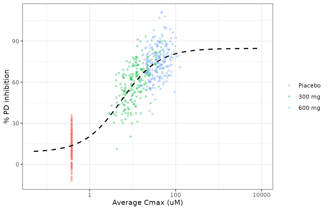
Replicates Figure 3 of Perello 2024: typical-value curve with simulated subjects.
Exposure-efficacy model: change in log CAC volume
Gate 3 – back-transformed Table 5 values
Table 5 reports E0 and Emax back-transformed as
100 * (exp(theta) - 1). With the Emax = -E0
constraint, the log-scale curve starts at e0 and decays to
zero, and the reported EC80 is 4 * EC50.
predEff <- function(cmax) {
  d <- data.frame(id = seq_along(cmax), time = 0, evid = 0, amt = 0, CMAX = cmax)
  suppressWarnings(rxode2::rxSolve(rxode2::zeroRe(uiEff), d, returnType = "data.frame"))$lncacvolcfb
}
pct <- function(x) 100 * (exp(x) - 1)
e0Log <- predEff(0)
ec50Eff <- 12.2
ec80Eff <- stats::uniroot(function(x) predEff(x) - 0.2 * e0Log, c(1, 500))$root

gate3 <- data.frame(
  Quantity = c("E0, % CAC change", "Emax, % CAC change", "EC80 (uM)"),
  Published = c(16.9, -14.5, 48.7),
  Model = c(pct(e0Log), pct(-e0Log), ec80Eff)
)
knitr::kable(gate3, digits = 2, caption = "Gate 3: Table 5 back-transformed estimates.")| Quantity | Published | Model |
|---|---|---|
| E0, % CAC change | 16.9 | 16.90 |
| Emax, % CAC change | -14.5 | -14.46 |
| EC80 (uM) | 48.7 | 48.80 |
Gate 4 – Figure 4B quartile means
Figure 4B labels the observed mean percent change in CAC volume for each Cmax quartile (placebo and four quartiles of the treated patients). The model curve should pass within the standard-error bars of those means.
quart <- data.frame(
  `Quartile mean Cmax (uM)` = c(0.4, 9.0, 17.4, 32.0, 60.1),
  `Observed % change` = c(15.9, 11.3, 6.5, 3.3, 2.6),
  check.names = FALSE
)
quart$`Model % change` <- pct(predEff(quart$`Quartile mean Cmax (uM)`))
quart$`Difference (pp)` <- quart$`Model % change` - quart$`Observed % change`
knitr::kable(quart, digits = 2, caption = "Gate 4: model curve vs Figure 4B quartile means.")| Quartile mean Cmax (uM) | Observed % change | Model % change | Difference (pp) |
|---|---|---|---|
| 0.4 | 15.9 | 16.32 | 0.42 |
| 9.0 | 11.3 | 9.40 | -1.90 |
| 17.4 | 6.5 | 6.65 | 0.15 |
| 32.0 | 3.3 | 4.40 | 1.10 |
| 60.1 | 2.6 | 2.67 | 0.07 |
Figure 4B and a simulated cohort
The same 600-subject cohort is passed through the efficacy model.
rxode2::rxSetSeed(20242)
simEff <- suppressWarnings(rxode2::rxSolve(uiEff, cohort, returnType = "data.frame", keep = "arm"))
simEff$pctChange <- pct(simEff$sim)

effArm <- simEff |>
  group_by(arm) |>
  summarise(
    `Typical % change at arm median Cmax` = pct(predEff(stats::median(CMAX))),
    `Simulated median % change` = stats::median(pctChange),
    .groups = "drop"
  )
knitr::kable(effArm, digits = 1, caption = "Predicted week-52 percent change in CAC volume by arm.")| arm | Typical % change at arm median Cmax | Simulated median % change |
|---|---|---|
| Placebo | 16.4 | 15.1 |
| 300 mg | 8.3 | 8.5 |
| 600 mg | 3.7 | 3.2 |
# Ordering of the typical predictions is deterministic in the arm medians.
stopifnot(all(diff(effArm$`Typical % change at arm median Cmax`) < 0))
curve4 <- data.frame(CMAX = seq(0, 100, length.out = 201))
curve4$pct <- pct(predEff(curve4$CMAX))
ggplot() +
  geom_line(data = curve4, aes(CMAX, pct), linetype = "dashed", linewidth = 0.8) +
  geom_point(data = quart, aes(`Quartile mean Cmax (uM)`, `Observed % change`), size = 2.5, shape = 18) +
  labs(x = "Average Cmax (uM)", y = "% change from baseline in CAC volume") +
  theme_bw()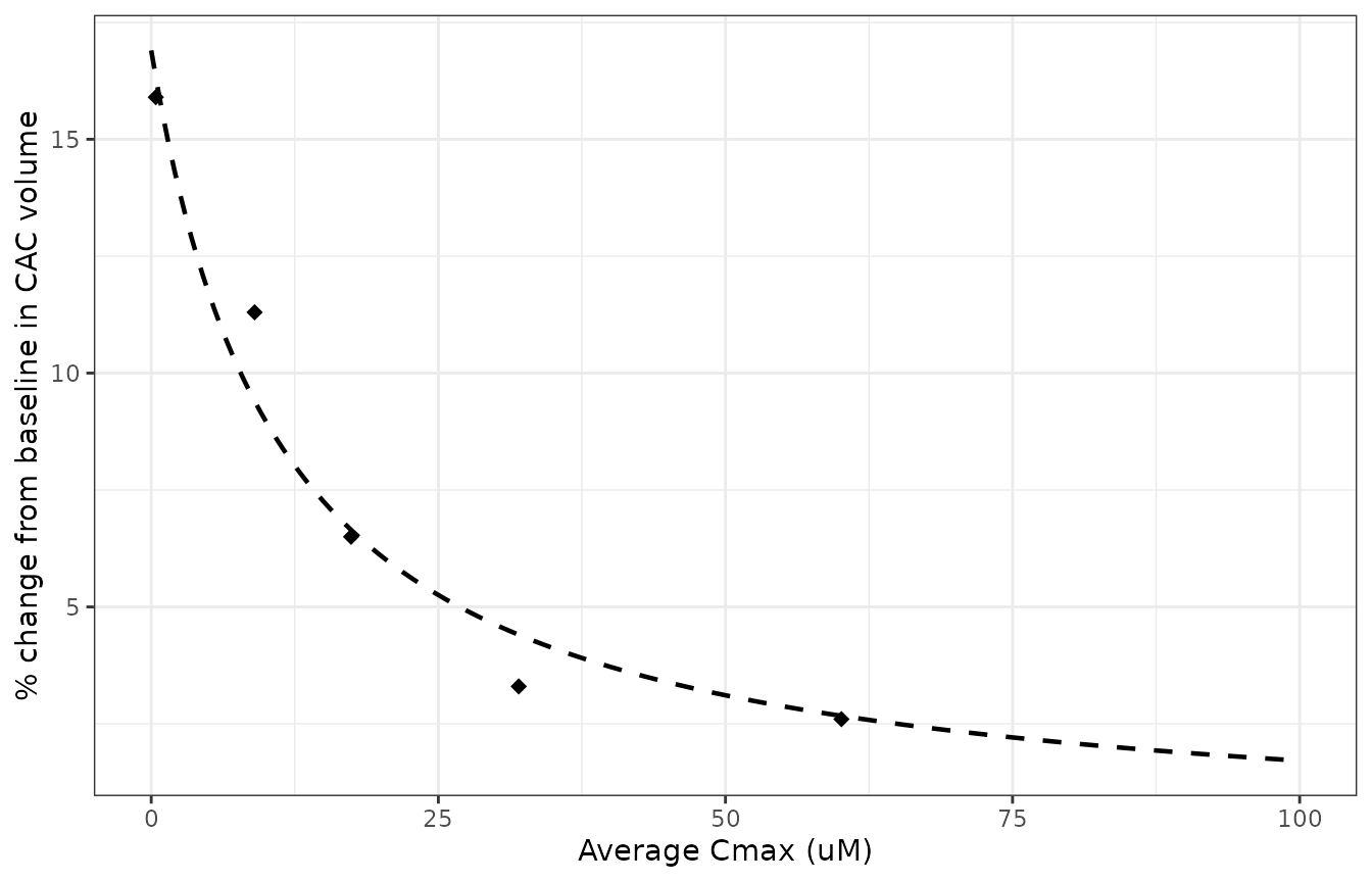
Replicates Figure 4B of Perello 2024: back-transformed model curve with the observed quartile means.
NCA
Neither model has a concentration-time course: the exposure is an observed end-of-infusion concentration supplied as data, and the outputs are subject-level averages or a single week-52 change. There is therefore nothing for PKNCA to compute, and the exposure gates above take its place.
Assumptions and deviations
- Baseline log CAC volume term omitted. The published efficacy model was “adjusted by baseline log CAC volume” (Results 3.5; it is the third model degree of freedom in Table 5), but neither the coefficient nor its centring value is reported, and there is no supplement. The packaged model is the curve with that term at its centring value, which is the “Model Estimates” line of Figure 4B. Individual predictions for patients far from the typical baseline will be biased by an unknown amount.
-
Log-scale E0 back-solved. Table 5 prints only
back-transformed values.
e0 = log(1.169); the log-scale confidence intervals of E0 and Emax are exact mirror images and both rows carry t = 3.39, confirmingEmax = -E0on the log scale. -
Residual SDs from the ANOVA tables. The PK/PD SD is
sqrt(126.4). The efficacy SD issqrt(1.4 / 53), where the error sum of squares is printed to one decimal place, so it is known only to about +/- 0.003. - Table 5 observation count. Table 5 implies 56 observations (Model DF 3 + Error DF 53, uncorrected total) while Results 3.1 report 55 per-protocol patients; the paper does not explain the difference.
-
Quartile labels vs model predictions. Results 3.5
call 3.3 % and 2.6 % the “predicted CAC progression rates” at the third
and fourth Cmax quartiles, but in Figure 4B those numbers are the
observed quartile means. The model curve gives 4.4 % and 2.7 % at those
Cmax values. Similarly, the paper’s “2.4 % progression at maximal
effect” is the arithmetic difference 16.9 - 14.5 of the back-transformed
values; under
Emax = -E0the modelled progression tends to 0 % at saturating exposure. - Virtual-cohort exposure. Average Cmax is drawn log-normally from the Table 2 arm mean and SD; the paper does not report its distribution beyond the Figure 3 and 4 box plots.
- No random effects. Methods 2.3 describe a mixed-effects framework, but the final models have one record per subject (55 observations, error DF 52 in Table 3), so they are packaged as typical-value regressions with an additive residual.
- BLQ handling. Concentrations below 0.758 uM were set to 0.379 uM (LQ/2). Table 4’s sensitivity fits (BLQ = 0 or BLQ = LQ) gave EC50 values of 6.33 and 4.66 uM; the packaged values are the primary LQ/2 fit.