Cladribine (Lindemalm 2005)
Source:vignettes/articles/Lindemalm_2005_cladribine.Rmd
Lindemalm_2005_cladribine.RmdModel and source
- Citation: Lindemalm S, Savic RM, Karlsson MO, Juliusson G, Liliemark J, Albertioni F. Application of population pharmacokinetics to cladribine. BMC Pharmacol. 2005;5:4. doi:10.1186/1471-2210-5-4. PMID: 15757511; PMCID: PMC1079880.
- Description: Three-compartment population PK model for cladribine (2-chlorodeoxyadenosine) in adults with indolent lymphoid and myeloid malignancies (Lindemalm 2005), pooled across intravenous infusion, oral solution and subcutaneous injection: first-order absorption from separate oral (F = 0.353) and subcutaneous (F = 1 fixed) depots, exponential IIV with one variance shared by Q2, Q3 and V3, and route-specific proportional residual error with between-subject variability on the residual magnitude. No covariates retained.
- Article: https://doi.org/10.1186/1471-2210-5-4 (open access, PMC1079880)
Lindemalm 2005 is a retrospective NONMEM (FOCE with interaction)
analysis of cladribine plasma concentrations pooled from five earlier
Swedish and British PK studies in which the drug was given as a 2-hour
or continuous intravenous infusion, as an oral solution, or as a
subcutaneous injection. One integrated model fits all three routes. The
later multiple-sclerosis model of the same drug,
Savic_2017_cladribine, is a separate analysis of a
different population and dataset.
Population
The final analysis used 1102 plasma concentrations from 168 courses in 161 patients (Lindemalm 2005 Methods, Patients). Table 1 of the paper describes the 163 patients initially included: 129 men and 34 women, mean age 60 years (range 22-89), mean weight 76 kg (48-118), mean height 174 cm (152-198) and mean body surface area 1.9 m^2 (1.5-2.4). Diagnoses were hairy cell leukaemia (84), chronic lymphocytic leukaemia (63), non-Hodgkin lymphoma (7), chronic myeloid leukaemia (4), acute myeloid leukaemia (3) and Langerhans cell histiocytosis (2). Mean Cockcroft-Gault creatinine clearance was 81 mL/min (Table 2); no patient had severe renal or hepatic impairment.
Doses (Methods, Drug administration) were 5 mg/m^2 (or 0.12 mg/kg) as a 2-hour IV infusion, 10 mg/m^2 (or 0.24 mg/kg) as an oral solution after an overnight fast, and 5 mg/m^2 subcutaneously into the abdominal wall. Six patients received a continuous IV infusion of 4.0-5.6 mg/m^2/24 h for 4-7 days. The infusion data came from 93 doses, the subcutaneous data from 83 doses and the oral data from 24 doses; seven patients contributed both IV and oral data.
The same information is available programmatically via
readModelDb("Lindemalm_2005_cladribine")()$population.
Source trace
Every value below is from Lindemalm 2005 Table 3 unless stated otherwise.
| Equation / parameter | Value | Source location |
|---|---|---|
lcl (CL) |
39.3 L/h | Table 3 (RSE 4.9%) |
lvc (V1) |
71.7 L | Table 3 (RSE 13%) |
lq (Q2) |
51.1 L/h | Table 3 (RSE 6.8%) |
lvp (V2) |
475 L | Table 3 (RSE 1.8%) |
lq2 (Q3) |
105 L/h | Table 3 (RSE 21%) |
lvp2 (V3) |
73.6 L | Table 3 (RSE 13%) |
lka_oral |
1.31 1/h | Table 3 ‘Oral Ka’; Results |
lfdepot_oral |
0.353 | Table 3 ‘Oral F’; Results |
lka_sc |
2.48 1/h | Table 3 ‘Subcutaneous Ka’; Results |
lfdepot_sc |
1 (fixed) | Results: subcutaneous F ‘was fixed to this value’ |
etalcl |
54% CV | Table 3 IIV |
etalvc |
34% CV | Table 3 IIV |
etalq (shared by Q2, Q3, V3) |
61% CV | Table 3 IIV, identical for Q2, Q3 and V3 |
etalvp |
70% CV | Table 3 IIV |
etalka_oral |
75% CV | Table 3 IIV |
etalfdepot_oral |
4.1% CV | Table 3 IIV; Results (‘4 %’) |
propSdIv / propSdOral /
propSdSc
|
0.191 / 0.232 / 0.162 | Table 3 residual error, footnote 2 |
etapropSd |
24% CV | Table 3 ‘IIV’ of residual error, footnote 3 |
| Three-compartment disposition, first-order absorption without lag | n/a | Results; Methods, Structural pharmacokinetic model |
| Exponential IIV | n/a | Methods, Statistical model |
| Route-specific proportional residual error with IIV on its magnitude | n/a | Methods, Statistical model (Karlsson 1995 method, ref 19) |
Cc in nmol/L |
n/a | Methods (assay LOQ 1 nM); Figures 1-3 axes |
Typical-value checks against the reported half-lives
The paper reports the half-lives of the three disposition phases
(0.2, 1.3 and 16 h; Results) and the share of the IV AUC carried by each
phase (11%, 24% and 65%; Discussion). Both follow from the Table 3
typical parameters alone, so they are checked exactly from the model’s
ini() values.
mod <- readModelDb("Lindemalm_2005_cladribine")
th <- rxode2::rxode(mod)$theta
#> ℹ parameter labels from comments will be replaced by 'label()'
cl <- exp(th[["lcl"]])
vc <- exp(th[["lvc"]])
q <- exp(th[["lq"]])
vp <- exp(th[["lvp"]])
q2 <- exp(th[["lq2"]])
vp2 <- exp(th[["lvp2"]])

kmat <- matrix(
  c(
    -(cl + q + q2) / vc, q / vp, q2 / vp2,
    q / vc, -q / vp, 0,
    q2 / vc, 0, -q2 / vp2
  ),
  nrow = 3, byrow = TRUE
)
ev <- eigen(kmat)
lambda <- -ev$values
# Coefficients of a unit IV bolus into central (amount scale), then the AUC
# carried by each exponential phase.
coef <- ev$vectors[1, ] * solve(ev$vectors, c(1, 0, 0))
auc_share <- (coef / lambda) / sum(coef / lambda)
ord <- order(lambda, decreasing = TRUE)

phase_tab <- tibble::tibble(
  Phase = c("First distribution", "Second distribution", "Terminal"),
  `t1/2 model (h)` = signif(log(2) / lambda[ord], 3),
  `t1/2 paper (h)` = c(0.2, 1.3, 16),
  `AUC share model (%)` = round(100 * auc_share[ord], 1),
  `AUC share paper (%)` = c(11, 24, 65)
)
knitr::kable(phase_tab, caption = "Disposition phases of the typical patient (Lindemalm 2005 Results and Discussion).")| Phase | t1/2 model (h) | t1/2 paper (h) | AUC share model (%) | AUC share paper (%) |
|---|---|---|---|---|
| First distribution | 0.189 | 0.2 | 10.5 | 11 |
| Second distribution | 1.280 | 1.3 | 24.8 | 24 |
| Terminal | 16.400 | 16.0 | 64.6 | 65 |
# Deterministic: the reported half-lives are rounded to the digits shown and the
# AUC shares to whole percent.
stopifnot(
  abs(log(2) / lambda[ord][1] - 0.2) < 0.05,
  abs(log(2) / lambda[ord][2] - 1.3) < 0.05,
  abs(log(2) / lambda[ord][3] - 16) < 0.5,
  all(abs(100 * auc_share[ord] - c(11, 24, 65)) < 1.5)
)
Virtual cohort
Original observed data are not publicly available. Each virtual patient draws a body surface area from a normal distribution with the Table 1 mean and SD (1.9 +/- 0.2 m^2), truncated to the reported 1.5-2.4 m^2 range, and receives the per-m^2 dose of their arm. Three single-dose arms of 200 patients each are simulated (2-hour IV infusion 5 mg/m^2, oral solution 10 mg/m^2, SC injection 5 mg/m^2), sampled densely through 168 h so a terminal half-life and an AUC to infinity can be estimated for each patient.
ROUTE_ORAL and ROUTE_IV are set on every
row from the arm’s route; the model reads them only to pick the
route-specific residual error.
rxode2::rxSetSeed(1079880)
set.seed(1079880)

obs_times <- c(
  0, 0.25, 0.5, 1, 1.5, 2, 2.25, 2.5, 3, 4, 5, 6, 8, 10, 12, 16, 20, 24,
  30, 36, 48, 60, 72, 96, 120, 144, 168
)

make_arm <- function(n, arm, dose_per_m2, id_offset) {
  bsa <- pmin(pmax(rnorm(n, 1.9, 0.2), 1.5), 2.4)
  cmt_dose <- switch(arm,
    IV = "central",
    Oral = "depot_oral",
    SC = "depot_sc"
  )
  subj <- tibble::tibble(
    id = id_offset + seq_len(n),
    arm = arm,
    BSA = bsa,
    ROUTE_ORAL = as.integer(arm == "Oral"),
    ROUTE_IV = as.integer(arm == "IV")
  )
  dose <- subj |>
    dplyr::mutate(
      time = 0, evid = 1L, cmt = cmt_dose, amt = dose_per_m2 * BSA,
      rate = dplyr::if_else(arm == "IV", amt / 2, 0)
    )
  obs <- subj |>
    tidyr::crossing(time = obs_times) |>
    dplyr::mutate(evid = 0L, cmt = "central", amt = 0, rate = 0)
  dplyr::bind_rows(dose, obs) |>
    dplyr::arrange(id, time, dplyr::desc(evid))
}

events <- dplyr::bind_rows(
  make_arm(200, "IV", 5, id_offset = 0L),
  make_arm(200, "Oral", 10, id_offset = 200L),
  make_arm(200, "SC", 5, id_offset = 400L)
)
stopifnot(!anyDuplicated(unique(events[, c("id", "time", "evid")])))
Simulation
sim <- rxode2::rxSolve(mod, events = events, keep = c("arm", "BSA")) |>
  as.data.frame()
#> ℹ parameter labels from comments will be replaced by 'label()'

mod_typical <- mod |> rxode2::zeroRe()
#> ℹ parameter labels from comments will be replaced by 'label()'
#> Warning: No sigma parameters in the model
events_typical <- events |>
  dplyr::filter(id %in% c(1L, 201L, 401L)) |>
  dplyr::mutate(
    amt = dplyr::if_else(evid == 1L, dplyr::if_else(arm == "Oral", 10, 5) * 1.9, 0),
    rate = dplyr::if_else(evid == 1L & arm == "IV", amt / 2, 0)
  )
sim_typical <- rxode2::rxSolve(
  mod_typical,
  events = events_typical, keep = c("arm"),
  rtol = 1e-10, atol = 1e-12
) |>
  as.data.frame()
#> ℹ omega/sigma items treated as zero: 'etalcl', 'etalvc', 'etalq', 'etalvp', 'etalka_oral', 'etalfdepot_oral', 'etapropSd'
#> Warning: multi-subject simulation without without 'omega'
Replicate published figures
Figure 1: concentration-time profiles by route
Figure 1 of the paper pools the observed concentrations of all three routes on a natural-log axis (log nmol/L from about 0 to 6 over the first 100 h). The simulated 5th, 50th and 95th percentiles per route are drawn on the same axis.
sim |>
  dplyr::filter(time %in% obs_times[obs_times > 0 & obs_times <= 100]) |>
  dplyr::group_by(arm, time) |>
  dplyr::summarise(
    Q05 = quantile(Cc, 0.05),
    Q50 = quantile(Cc, 0.50),
    Q95 = quantile(Cc, 0.95),
    .groups = "drop"
  ) |>
  ggplot(aes(time, log(Q50))) +
  geom_ribbon(aes(ymin = log(Q05), ymax = log(Q95), fill = arm), alpha = 0.2) +
  geom_line(aes(colour = arm)) +
  coord_cartesian(ylim = c(-0.5, 6.5)) +
  labs(
    x = "Time after dose (h)", y = "Log (concentration) (nmol/L)",
    colour = "Route", fill = "Route",
    title = "Simulated cladribine profiles, median and 90% interval",
    caption = "Compare with Figure 1 of Lindemalm 2005 (single doses: 2-h IV 5 mg/m^2, oral 10 mg/m^2, SC 5 mg/m^2)."
  )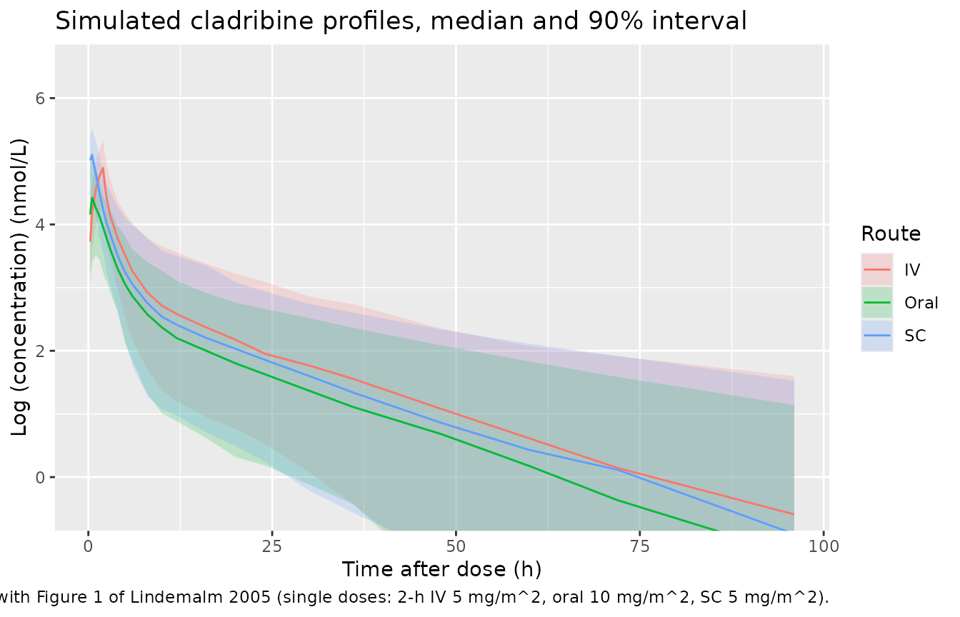
The simulated peaks after the 2-hour infusion and the SC injection sit at about log 4.5-5.5 and the 24-hour concentrations at about log 1-3, which is the band the observed points occupy in Figure 1.
Figure 2: continuous intravenous infusion
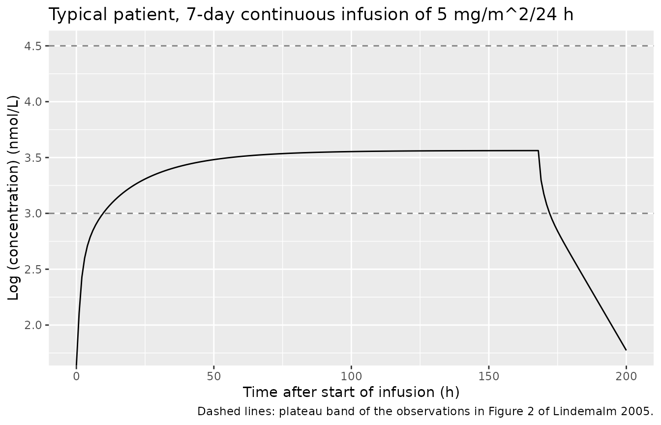
Figure 2 shows the observations from repeated and continuous IV
administration; the plateau points between roughly 50 and 170 h lie
between about log 3 and log 4.5 nmol/L. For the typical patient a
continuous infusion of 5 mg/m^2/24 h at 1.9 m^2 gives the steady state
R0 / CL.
r0 <- 5 * 1.9 / 24 # mg/h
ev_inf <- rxode2::et(amt = 5 * 1.9 * 7, rate = r0, cmt = "central") |>
  rxode2::et(seq(0, 200, by = 1)) |>
  as.data.frame() |>
  dplyr::mutate(ROUTE_ORAL = 0L, ROUTE_IV = 1L)
sim_inf <- rxode2::rxSolve(mod_typical, events = ev_inf, rtol = 1e-10, atol = 1e-12) |>
  as.data.frame()
#> ℹ omega/sigma items treated as zero: 'etalcl', 'etalvc', 'etalq', 'etalvp', 'etalka_oral', 'etalfdepot_oral', 'etapropSd'

css_expected <- r0 / cl * 1e6 / 285.69 # nmol/L
css_sim <- sim_inf$Cc[sim_inf$time == 160]

ggplot(sim_inf, aes(time, log(Cc))) +
  geom_line() +
  geom_hline(yintercept = c(3, 4.5), linetype = "dashed", colour = "grey50") +
  labs(
    x = "Time after start of infusion (h)", y = "Log (concentration) (nmol/L)",
    title = "Typical patient, 7-day continuous infusion of 5 mg/m^2/24 h",
    caption = "Dashed lines: plateau band of the observations in Figure 2 of Lindemalm 2005."
  )
# Deterministic: after 160 h (10 terminal half-lives) the solve is at
# R0/CL; the plateau lies inside the band read from Figure 2.
stopifnot(
  abs(css_sim / css_expected - 1) < 0.01,
  log(css_expected) > 3, log(css_expected) < 4.5
)
c(css_nmol_L = css_expected, log_css = log(css_expected))
#> css_nmol_L    log_css
#>  35.255329   3.562617
PKNCA validation
Clearance and bioavailability are the quantities the paper reports for each route. PKNCA estimates the AUC to infinity and the terminal half-life per patient; clearance (or CL/F) is the dose in nmol divided by the AUC.
# Integrator undershoot below zero is noise of order atol; assert that, then
# floor it so PKNCA does not take the log of a negative value.
stopifnot(all(sim$Cc >= -1e-6 * max(sim$Cc, na.rm = TRUE), na.rm = TRUE))
conc <- sim |>
  dplyr::filter(!is.na(Cc)) |>
  dplyr::mutate(Cc = pmax(Cc, 0)) |>
  dplyr::select(id, time, Cc, arm)
dose_df <- events |>
  dplyr::filter(evid == 1L) |>
  dplyr::select(id, time, amt, arm)

conc_obj <- PKNCA::PKNCAconc(conc, Cc ~ time | arm + id)
dose_obj <- PKNCA::PKNCAdose(dose_df, amt ~ time | arm + id)
intervals <- data.frame(
  start = c(0, 0),
  end = c(Inf, 24),
  cmax = c(TRUE, FALSE),
  tmax = c(TRUE, FALSE),
  aucinf.obs = c(TRUE, FALSE),
  half.life = c(TRUE, FALSE),
  auclast = c(FALSE, TRUE)
)
nca_res <- PKNCA::pk.nca(PKNCA::PKNCAdata(conc_obj, dose_obj, intervals = intervals))

nca_wide <- as.data.frame(nca_res) |>
  dplyr::filter(PPTESTCD %in% c("aucinf.obs", "half.life", "auclast", "cmax")) |>
  dplyr::mutate(PPTESTCD = dplyr::if_else(PPTESTCD == "auclast", "auc24", PPTESTCD)) |>
  dplyr::select(id, arm, PPTESTCD, PPORRES) |>
  tidyr::pivot_wider(names_from = PPTESTCD, values_from = PPORRES) |>
  dplyr::left_join(dose_df |> dplyr::select(id, amt), by = "id") |>
  dplyr::mutate(
    # CL (IV) or CL/F (oral, SC) in L/h: dose in nmol over AUC in nmol*h/L.
    cl.obs = amt * 1e6 / 285.69 / aucinf.obs,
    # Accumulation index for once-daily dosing: AUC over a steady-state
    # dosing interval / AUC over the first interval = AUCinf / AUC0-24.
    accum = aucinf.obs / auc24
  )
Comparison against published values
The reference values are the final-model CL (39.3 L/h) for the IV
arm, the apparent oral clearance from the paper’s route-specific
supplementary fit (105 L/h; Results), the final-model CL / F for the SC
arm (39.3 L/h with F fixed at 1), and the 16-hour terminal half-life
(Results). ncaComparisonTable() reports the median across
patients.
published <- tibble::tribble(
  ~arm, ~cl.obs, ~half.life,
  "IV", 39.3, 16,
  "Oral", 105, 16,
  "SC", 39.3, 16
)
sim_long <- nca_wide |>
  dplyr::select(arm, cl.obs, half.life) |>
  tidyr::pivot_longer(c(cl.obs, half.life), names_to = "PPTESTCD", values_to = "PPORRES")

cmp <- nlmixr2lib::ncaComparisonTable(
  simulated = sim_long,
  reference = published,
  by = "arm",
  units = c(cl.obs = "L/h", half.life = "h"),
  tolerance_pct = 20
)
knitr::kable(cmp, caption = "Simulated (median) vs. published clearance and terminal half-life. * differs from reference by >20%.")| NCA parameter | arm | Reference | Simulated | % diff |
|---|---|---|---|---|
| t½ (h) | IV | 16 | 18.7 | +16.7% |
| t½ (h) | Oral | 16 | 19 | +18.9% |
| t½ (h) | SC | 16 | 19 | +18.8% |
| CL/F (L/h) | IV | 39.3 | 38 | -3.3% |
| CL/F (L/h) | Oral | 105 | 118 | +11.9% |
| CL/F (L/h) | SC | 39.3 | 41.3 | +5.2% |
The median clearance of a cohort with 54% CV IIV on CL sits close to the typical value because clearance is log-normal, and the oral CL/F matches the paper’s separately estimated 105 L/h (39.3 / 0.353 = 111 L/h in the final model). The PKNCA half-life is fitted to each patient’s terminal points within 168 h and is the median across patients, so it carries the IIV of every disposition parameter on top of the typical 16 h.
med <- nca_wide |>
  dplyr::group_by(arm) |>
  dplyr::summarise(
    cl = median(cl.obs), thalf = median(half.life, na.rm = TRUE),
    accum_q10 = quantile(accum, 0.1, na.rm = TRUE),
    accum_q50 = median(accum, na.rm = TRUE),
    accum_q90 = quantile(accum, 0.9, na.rm = TRUE),
    .groups = "drop"
  )
knitr::kable(med, digits = 2, caption = "Per-arm medians and accumulation-index quantiles.")| arm | cl | thalf | accum_q10 | accum_q50 | accum_q90 |
|---|---|---|---|---|---|
| IV | 38.00 | 18.68 | 1.09 | 1.32 | 1.96 |
| Oral | 117.52 | 19.03 | 1.11 | 1.31 | 2.05 |
| SC | 41.33 | 19.02 | 1.09 | 1.31 | 1.91 |
# Typical-value bioavailability: dose-normalised AUC ratio against the IV arm.
auc_typ <- sim_typical |>
  dplyr::group_by(arm) |>
  dplyr::summarise(
    auc = sum(diff(time) * (head(Cc, -1) + tail(Cc, -1)) / 2),
    .groups = "drop"
  )
f_oral_typ <- (auc_typ$auc[auc_typ$arm == "Oral"] / 19) / (auc_typ$auc[auc_typ$arm == "IV"] / 9.5)
f_oral_typ
#> [1] 0.3511739

stopifnot(
  # Structural: a mis-transcribed CL, F or unit moves these medians by tens
  # of percent. Bands are wide enough for cohort-to-cohort variation of the
  # median of 200 log-normal draws (SE ~4%).
  abs(med$cl[med$arm == "IV"] / 39.3 - 1) < 0.15,
  abs(med$cl[med$arm == "Oral"] / (39.3 / 0.353) - 1) < 0.15,
  abs(med$cl[med$arm == "SC"] / 39.3 - 1) < 0.15,
  # Trapezoidal typical-value F over a 168-h grid: within 5% of 0.353.
  abs(f_oral_typ / 0.353 - 1) < 0.05
)
Accumulation index
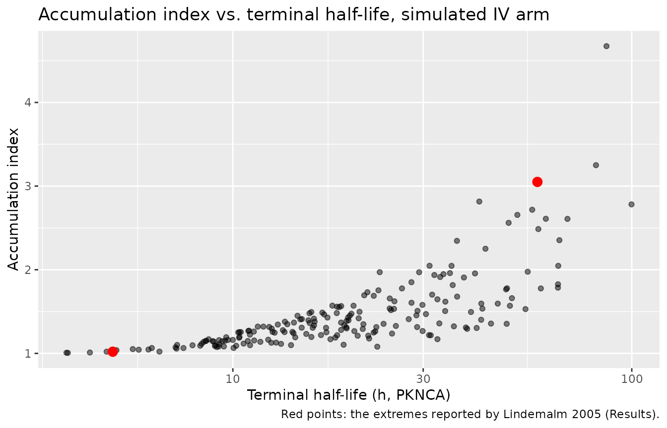
The paper reports an accumulation index between 1.02 and 3.05 for
repeated IV dosing (the extremes, for the patients with the shortest and
longest terminal half-lives of 5 and 58 h; Results). In the simulated IV
arm the index is AUCinf / AUC0-24 after a single infusion,
which equals the steady-state to first-interval AUC ratio for once-daily
dosing.
iv_acc <- nca_wide |> dplyr::filter(arm == "IV")
ggplot(iv_acc, aes(half.life, accum)) +
  geom_point(alpha = 0.5) +
  annotate("point", x = c(5, 58), y = c(1.02, 3.05), colour = "red", size = 3) +
  scale_x_log10() +
  labs(
    x = "Terminal half-life (h, PKNCA)", y = "Accumulation index",
    title = "Accumulation index vs. terminal half-life, simulated IV arm",
    caption = "Red points: the extremes reported by Lindemalm 2005 (Results)."
  )
# The reported range spans 161 patients; the central 80% of the simulated
# cohort must lie inside it.
stopifnot(
  med$accum_q10[med$arm == "IV"] > 1.02,
  med$accum_q90[med$arm == "IV"] < 3.05
)
Assumptions and deviations
-
Shared eta on Q2, Q3 and V3. Table 3 reports the
same IIV (61%) with the same RSE (17%) for Q2, Q3 and V3. The
maintainers read this as one random effect shared by the three
parameters (one NONMEM ETA), which reproduces the reported marginal CV
of each. Three independent random effects constrained to one variance
(
$OMEGA BLOCK(1) SAME) would give the same marginal CVs but no correlation between them; the paper does not say which was used. -
CV to variance. Table 3 gives IIV as a coefficient
of variation; the log-normal variances are
log(1 + CV^2). -
Residual error scale. The Table 3 residual-error
values (0.191, 0.232, 0.162) are read as proportional standard
deviations (fractions), consistent with the table’s other variability
terms being on the CV scale. The 24% IIV in residual variability is an
exponential random effect on that SD
(
propSd * exp(etapropSd)), the implementation of the cited method (Karlsson 1995). - Molar mass. Concentrations are returned in nmol/L, the unit of the assay and of every figure in the paper, using the cladribine molar mass of 285.69 g/mol, which is not stated in the paper.
- No covariates. None of the screened covariates (sex, age, weight, height, BSA, creatinine clearance, liver tests, lymphocyte count, diagnosis) was retained, so the virtual cohort varies only BSA, and only to set the per-m^2 dose.
- Single-dose design. The paper’s courses were mostly once-daily infusions or injections over several days; the cohort here gives single doses so each route’s profile and NCA can be compared directly. The accumulation index is derived from the single-dose IV profile.
- Errata. No correction notice for this article was found in Europe PMC (checked 2026-10-29).