Ethaselen mouse dose-biomarker-response (Ye 2017)
Source:vignettes/articles/Ye_2017_ethaselen.Rmd
Ye_2017_ethaselen.RmdModel and source
- Citation: Ye SF, Li J, Ji SM, Zeng HH, Lu W. Dose-biomarker-response modeling of the anticancer effect of ethaselen in a human non-small cell lung cancer xenograft mouse model. Acta Pharmacologica Sinica 2017;38(2):223-232. doi:[10.1038/aps.2016.114](https://doi.org/10.1038/aps.2016.114).
- Article published online 5 December 2016; cited as Acta Pharmacologica Sinica (2017) 38:223-232.
This vignette validates the preclinical (mouse, A549 NSCLC xenograft) integrated dose-biomarker-response model for ethaselen. The structural model couples a thioredoxin-reductase (TrxR) indirect-response biomarker turnover to a smooth exponential-to-linear tumor-growth law, with a sigmoidal Emax dose effect inhibiting TrxR turnover and a simple Emax tumor-killing rate driven by the relative TrxR inhibition ratio P.
Population
132 BALB/c nude mice were used for the TrxR biomarker arm (4 dose groups x 33 mice; 3 mice sacrificed per day across the 10 dosing days plus follow-up) and 28 additional mice were used for the tumor-volume arm (4 dose groups x 7 mice; daily caliper measurements). The combined data set drives the integrated model. Mice received ethaselen by oral gavage (ig) at 0 (vehicle 0.5% CMC-Na), 36, 72, or 108 mg/kg once daily for 10 days; randomisation occurred when tumor volume reached approximately 100 mm^3. Source: Ye 2017 Methods.
The same information is available programmatically via
readModelDb("Ye_2017_ethaselen")$population.
Source trace
The integrated model is paper Equations 3-9; parameter values are
from Table 1. The model has no PK ODE – the paper acknowledges that
ethaselen plasma concentrations were not measured. Drug exposure enters
through the time-varying covariate DOSE (mg/kg/day).
| Equation / parameter | Value | Source location |
|---|---|---|
d/dt(trxr) |
n/a | Eq 4 (drug-modulated IDR; explicit form derived from prose, see Assumptions below) |
d/dt(trxr_ctrl) |
n/a | Shadow control state required by Eq 7 P-ratio definition |
d/dt(tumor_volume) |
n/a | Eq 8 (natural growth from Eq 5 minus simple Emax kill) |
Kin_eff = Kin*(1+gamma*growth_rate) |
n/a | Prose: “Kin was influenced by tumor growth rates with a linear correction factor” |
growth_rate = 2*lambda0*lambda1*X / (lambda1 + 2*lambda0*X) |
n/a | Eq 5 |
Kout_eff = Kout*(1 + Smax*DOSE^hill / (SC50^hill + DOSE^hill)) |
n/a | Prose: sigmoidal Emax on Kout with Smax / SC50 / Hill (gamma2) |
P = 1 - trxr / trxr_ctrl |
n/a | Eq 7 |
kill = Emax*P / (EC50 + P) |
n/a | Eq 8 |
lkin (Kin) |
log(8.27) |
Table 1: Kin = 8.27 U/mL/d (RSE 42.4%) |
lrbase (Base) |
log(39.7) |
Table 1: Base = 39.7 U/mL (RSE 8.6%) |
lgamma (gamma1) |
log(0.021) |
Table 1: gamma1 = 0.021 d/mm (RSE 16.5%) |
lsmax (Smax) |
log(5.95) |
Table 1: Smax = 5.95 (RSE 31.9%) |
lsc50 (SC50) |
log(136) |
Table 1: SC50 = 136 mg/kg (RSE 25.2%) |
lhill (gamma2) |
log(2.29) |
Table 1: gamma2 = 2.29 (RSE 17.3%) |
llambda0 |
log(0.704) |
Table 1: lambda0 = 0.704 /d (RSE 31.4%) |
llambda1 |
log(321) |
Table 1: lambda1 = 321 mm^3/d (RSE 11.5%) |
lrbase_tumor (W) |
log(103) |
Table 1: W = 103 mm^3 (RSE 3.9%) |
lemax |
log(130) |
Table 1: Emax = 130 mm^3/d (RSE 4.8%) |
lec50 |
log(0.0676) |
Table 1: EC50 = 0.0676 (RSE 23.1%) |
etalkin |
0.01526 |
Table 1: CV = 12.4% on Kin (omega^2 = log(0.124^2+1)) |
etalrbase |
0.00917 |
Table 1: CV = 9.6% on Base |
etallambda1 |
0.10160 |
Table 1: CV = 32.7% on lambda1 |
etalrbase_tumor |
0.01996 |
Table 1: CV = 14.2% on W |
etalec50 |
0.03657 |
Table 1: CV = 19.3% on EC50 |
propSd_tumor_volume |
0.2022 |
Table 1: Err_pro = 20.22% (RSE 13.6%) |
addSd_tumor_volume |
141 |
Table 1: Err_add = 141 mm^3 (RSE 78%) |
propSd_trxr |
0.2022 |
Inherited from Err_pro; paper does not separately report TrxR residual (assumption) |
Virtual cohort
The published study used 33 mice per dose group for the biomarker arm
and 7 mice per group for the tumor-volume arm. The virtual cohort below
pools both into 33 mice per group (132 mice total) for stochastic
simulation, and uses a smaller 10-mouse-per-group cohort for
typical-value plotting. Per-mouse initial tumor volume (W)
and the four IIV-bearing parameters are simulated by
rxode2::rxSolve’s built-in IIV machinery; the dose level is
provided as the time-varying DOSE covariate.
set.seed(2017)

dose_groups <- tibble::tribble(
  ~dose_mgkg, ~dose_label,
  0,          "0 mg/kg (vehicle)",
  36,         "36 mg/kg",
  72,         "72 mg/kg",
  108,        "108 mg/kg"
) |>
  mutate(dose_label = factor(dose_label,
                             levels = c("0 mg/kg (vehicle)",
                                        "36 mg/kg",
                                        "72 mg/kg",
                                        "108 mg/kg")))

obs_times <- seq(0, 14, by = 0.5)   # 0-10 d dosing window plus 4 d follow-up

make_cohort <- function(n_per_group, dose_mgkg, dose_label, id_offset) {
  ids <- id_offset + seq_len(n_per_group)
  per_subject <- tibble(id = ids, dose_label = dose_label)
  per_subject |>
    tidyr::crossing(time = obs_times) |>
    mutate(
      evid = 0L,
      amt  = 0,
      DOSE = ifelse(time < 10, dose_mgkg, 0)
    )
}

n_per_group <- 10L
events_typical <- bind_rows(
  make_cohort(n_per_group, dose_groups$dose_mgkg[1], dose_groups$dose_label[1], id_offset = 0L),
  make_cohort(n_per_group, dose_groups$dose_mgkg[2], dose_groups$dose_label[2], id_offset = 1L * n_per_group),
  make_cohort(n_per_group, dose_groups$dose_mgkg[3], dose_groups$dose_label[3], id_offset = 2L * n_per_group),
  make_cohort(n_per_group, dose_groups$dose_mgkg[4], dose_groups$dose_label[4], id_offset = 3L * n_per_group)
)

stopifnot(!anyDuplicated(unique(events_typical[, c("id", "time", "evid")])))
nrow(events_typical); n_distinct(events_typical$id)
#> [1] 1160
#> [1] 40
Typical-value simulation (Figure 4 left-side panels)
A typical-value simulation (zeroRe(): no IIV, no
residual error) reproduces the shape Ye 2017 Figure 4 panels A-D show
for the TrxR biomarker: control TrxR rises monotonically as the tumor
grows (Kin is linearly amplified by the natural growth rate), while
increasing ethaselen doses bend the trajectory downward.
mod <- readModelDb("Ye_2017_ethaselen")
mod_typ <- mod |> rxode2::zeroRe()
#> ℹ parameter labels from comments will be replaced by 'label()'

sim_typ <- rxode2::rxSolve(
  mod_typ,
  events = events_typical,
  keep   = c("DOSE", "dose_label")
) |>
  as.data.frame()
#> ℹ omega/sigma items treated as zero: 'etalkin', 'etalrbase', 'etallambda1', 'etalrbase_tumor', 'etalec50'
#> Warning: multi-subject simulation without without 'omega'

typ_summary <- sim_typ |>
  group_by(dose_label, time) |>
  summarise(median_trxr  = median(trxr),
            median_tumor = median(tumor_volume),
            median_p     = median(p_inhib),
            .groups = "drop")

ggplot(typ_summary, aes(time, median_trxr, colour = dose_label)) +
  geom_line(linewidth = 1) +
  geom_vline(xintercept = 10, linetype = "dashed", colour = "grey50") +
  labs(x = "Time (days)", y = "TrxR activity (U/mL)",
       colour = "Dose group",
       title = "Figure 4 A-D -- TrxR by dose (typical value)",
       caption = "Replicates Ye 2017 Figure 4 A-D shape. Dashed line marks end of dosing (day 10).") +
  theme_minimal()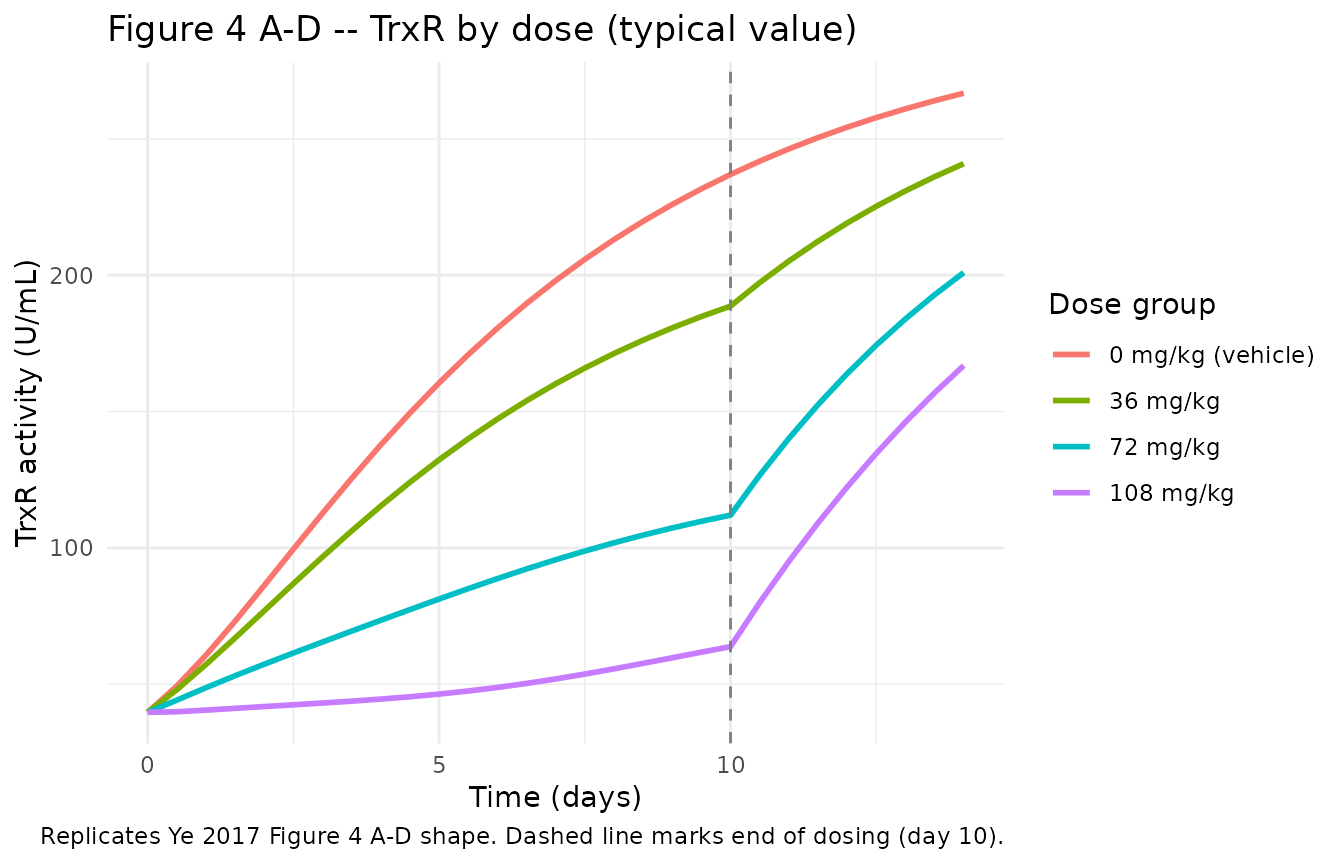
ggplot(typ_summary, aes(time, median_tumor, colour = dose_label)) +
  geom_line(linewidth = 1) +
  geom_vline(xintercept = 10, linetype = "dashed", colour = "grey50") +
  labs(x = "Time (days)", y = "Tumor volume (mm^3)",
       colour = "Dose group",
       title = "Figure 3B / Figure 4 E-H -- Tumor volume by dose (typical value)",
       caption = "Replicates Ye 2017 Figure 3B and Figure 4 E-H. Dashed line marks end of dosing.") +
  theme_minimal()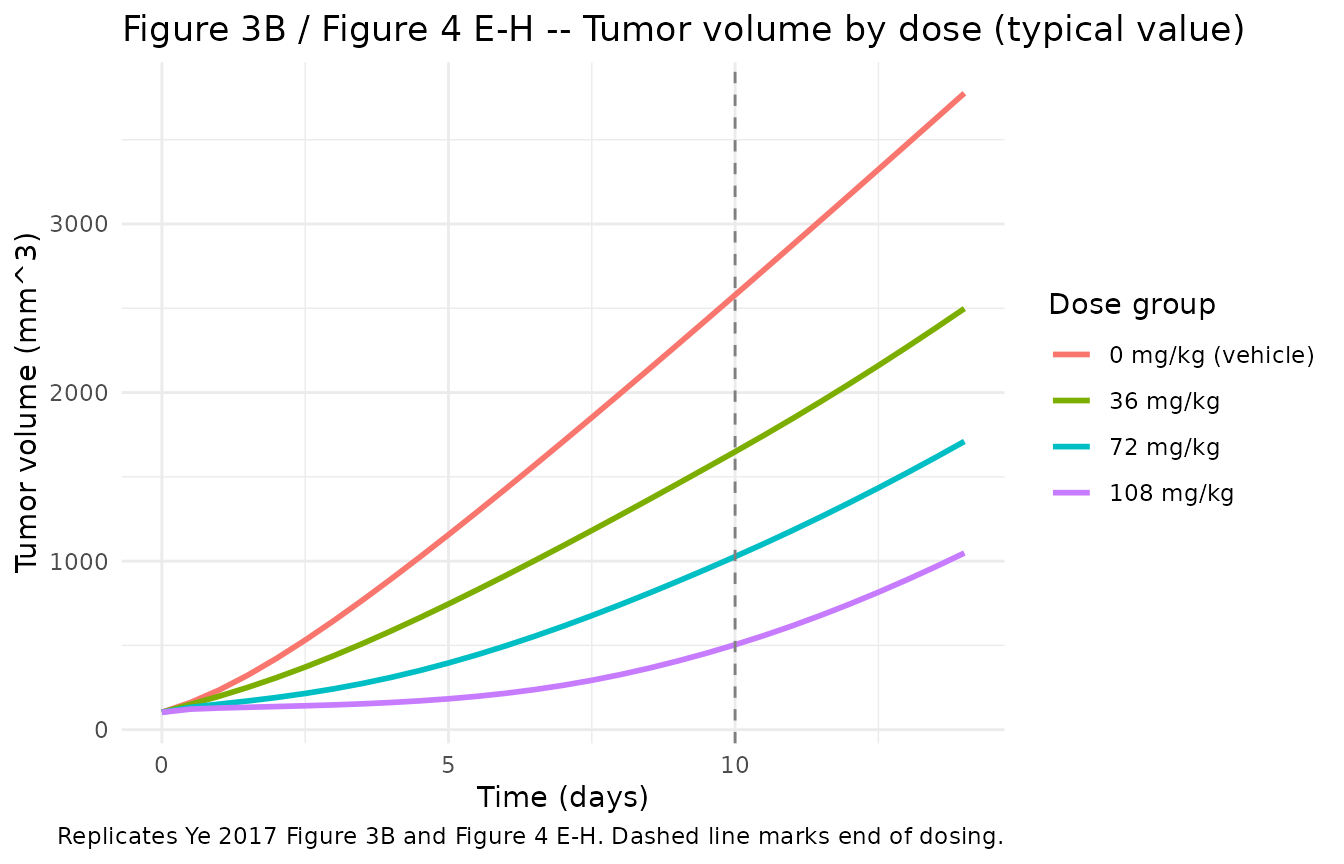
Stochastic simulation (Figure 7 VPC structure)
Including IIV on Kin / Base / lambda1 / W / EC50 plus the proportional + additive residual error reproduces the VPC structure of Ye 2017 Figure 7. The published VPC used 1000 simulated replicates per dose group; the cohort below uses 33 mice per group (matching the source N) and the model’s built-in IIV.
events_stoch <- bind_rows(
  make_cohort(33L, dose_groups$dose_mgkg[1], dose_groups$dose_label[1], id_offset = 0L),
  make_cohort(33L, dose_groups$dose_mgkg[2], dose_groups$dose_label[2], id_offset = 33L),
  make_cohort(33L, dose_groups$dose_mgkg[3], dose_groups$dose_label[3], id_offset = 66L),
  make_cohort(33L, dose_groups$dose_mgkg[4], dose_groups$dose_label[4], id_offset = 99L)
)
stopifnot(!anyDuplicated(unique(events_stoch[, c("id", "time", "evid")])))

sim_iiv <- rxode2::rxSolve(
  mod,
  events = events_stoch,
  keep   = c("DOSE", "dose_label")
) |>
  as.data.frame()
#> ℹ parameter labels from comments will be replaced by 'label()'
#> Warning: some ID(s) could not solve the ODEs correctly; These values are
#> replaced with 'NA'

vpc_trxr <- sim_iiv |>
  group_by(dose_label, time) |>
  summarise(
    Q10 = quantile(trxr, 0.10, na.rm = TRUE),
    Q50 = quantile(trxr, 0.50, na.rm = TRUE),
    Q90 = quantile(trxr, 0.90, na.rm = TRUE),
    .groups = "drop"
  )

ggplot(vpc_trxr, aes(time, Q50, colour = dose_label, fill = dose_label)) +
  geom_ribbon(aes(ymin = pmax(Q10, 0), ymax = Q90), alpha = 0.2, colour = NA) +
  geom_line(linewidth = 1) +
  geom_vline(xintercept = 10, linetype = "dashed", colour = "grey50") +
  facet_wrap(~ dose_label, ncol = 2, scales = "free_y") +
  labs(x = "Time (days)", y = "TrxR activity (U/mL)",
       title = "Figure 7 A-D -- VPC: 10/50/90 percentile bands for TrxR by dose",
       caption = "Replicates Ye 2017 Figure 7 A-D structure (80% prediction interval).") +
  theme_minimal() +
  guides(colour = "none", fill = "none")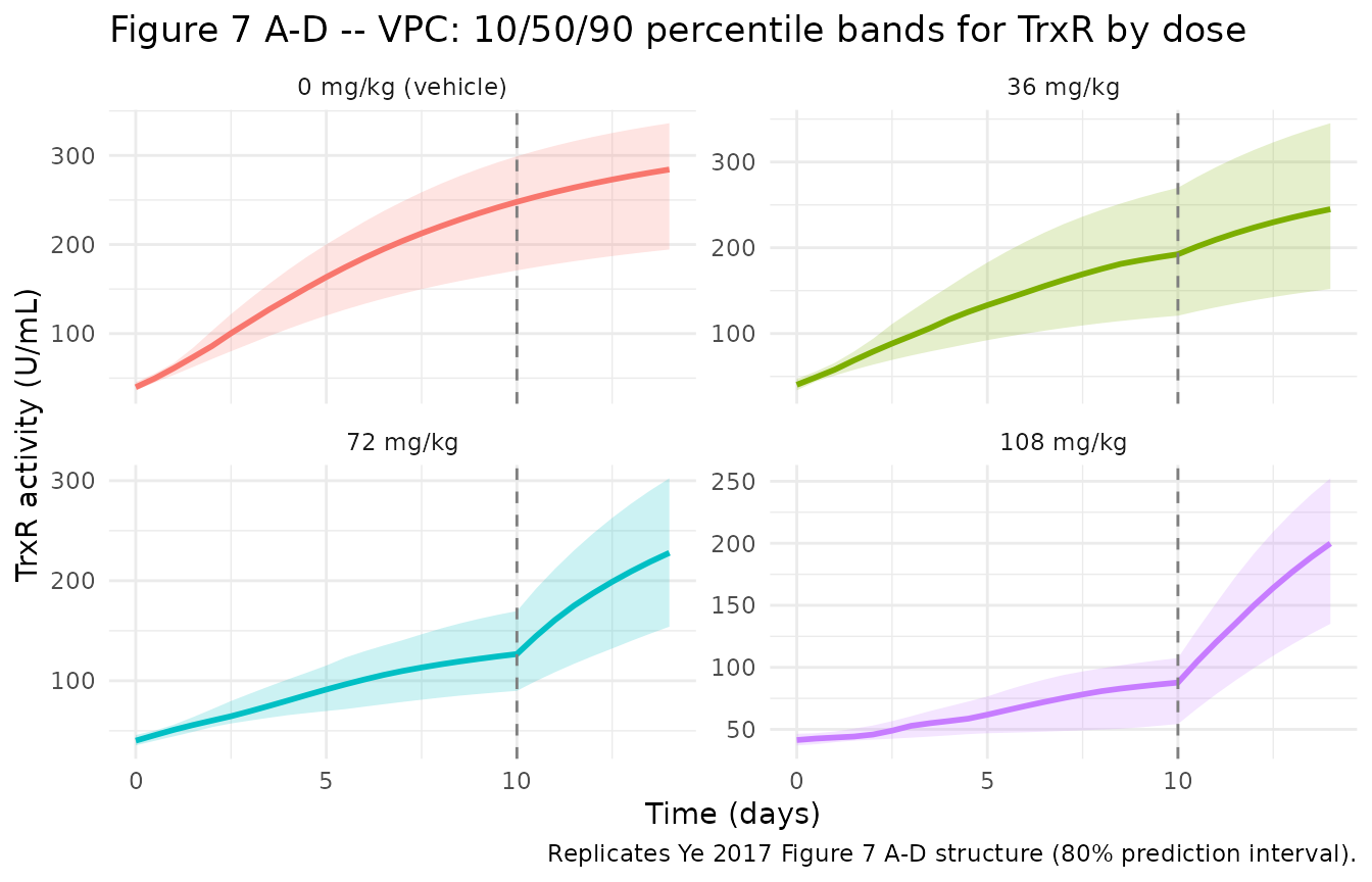
vpc_tumor <- sim_iiv |>
  group_by(dose_label, time) |>
  summarise(
    Q10 = quantile(tumor_volume, 0.10, na.rm = TRUE),
    Q50 = quantile(tumor_volume, 0.50, na.rm = TRUE),
    Q90 = quantile(tumor_volume, 0.90, na.rm = TRUE),
    .groups = "drop"
  )

ggplot(vpc_tumor, aes(time, Q50, colour = dose_label, fill = dose_label)) +
  geom_ribbon(aes(ymin = pmax(Q10, 0), ymax = Q90), alpha = 0.2, colour = NA) +
  geom_line(linewidth = 1) +
  geom_vline(xintercept = 10, linetype = "dashed", colour = "grey50") +
  facet_wrap(~ dose_label, ncol = 2, scales = "free_y") +
  labs(x = "Time (days)", y = "Tumor volume (mm^3)",
       title = "Figure 7 E-H -- VPC: 10/50/90 percentile bands for tumor volume by dose",
       caption = "Replicates Ye 2017 Figure 7 E-H structure (80% prediction interval).") +
  theme_minimal() +
  guides(colour = "none", fill = "none")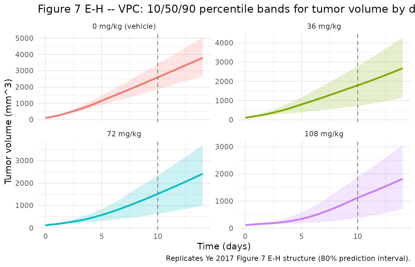
Mechanistic sanity checks
This is a PD-only dose-biomarker-response model with no drug-concentration time course, so PKNCA-based validation is not the right target (there is no concentration to integrate). The mechanistic checks below cover the failure modes that would actually break this class of model.
1. Vehicle arm: trxr equals trxr_ctrl, P = 0, no tumor killing
In the vehicle arm DOSE = 0 so
drug_effect = 0 and kout_eff = kout. The
trxr and trxr_ctrl states must therefore
coincide at every time point (both ODEs are identical),
P = 0, and the tumor grows according to the unmodified Eq
5.
veh_typ <- sim_typ |> filter(dose_label == "0 mg/kg (vehicle)")

# trxr and trxr_ctrl must be numerically equal in the vehicle arm
stopifnot(max(abs(veh_typ$trxr - veh_typ$trxr_ctrl)) < 1e-6)

# P must be exactly zero in the vehicle arm
stopifnot(max(veh_typ$p_inhib) < 1e-9)

# Tumor must grow monotonically (no killing)
stopifnot(all(diff(veh_typ$tumor_volume[veh_typ$id == veh_typ$id[1]]) >= 0))

knitr::kable(
  veh_typ |>
    filter(id == veh_typ$id[1], time %in% c(0, 2, 5, 7, 10, 14)) |>
    select(time, trxr, trxr_ctrl, p_inhib, tumor_volume),
  digits = 3,
  caption = "Vehicle arm -- trxr and trxr_ctrl coincide; P = 0; tumor grows naturally."
)| time | trxr | trxr_ctrl | p_inhib | tumor_volume |
|---|---|---|---|---|
| 0 | 39.700 | 39.700 | 0 | 103.000 |
| 2 | 86.220 | 86.220 | 0 | 422.962 |
| 5 | 160.487 | 160.487 | 0 | 1156.618 |
| 7 | 198.011 | 198.011 | 0 | 1709.540 |
| 10 | 236.933 | 236.933 | 0 | 2578.815 |
| 14 | 266.729 | 266.729 | 0 | 3775.884 |
2. Dose-response monotonicity in TrxR and tumor
Across the four dose groups, increasing dose should monotonically lower the TrxR trajectory and the tumor trajectory at any time point during the dosing window. This catches sign / form errors in the drug-effect equation.
day10 <- typ_summary |> filter(time == 10) |>
  arrange(dose_label) |>
  select(dose_label, median_trxr, median_tumor, median_p)

knitr::kable(day10, digits = 3,
caption = "Day-10 median (typical-value) trajectory by dose group.")| dose_label | median_trxr | median_tumor | median_p |
|---|---|---|---|
| 0 mg/kg (vehicle) | 236.933 | 2578.815 | 0.000 |
| 36 mg/kg | 188.653 | 1648.913 | 0.158 |
| 72 mg/kg | 111.994 | 1026.675 | 0.445 |
| 108 mg/kg | 63.801 | 504.019 | 0.614 |
3. Steady-state behaviour at zero tumor growth
If the tumor growth rate were zero (a hypothetical “frozen tumor”),
the Kin amplification term (1 + gamma * growth_rate) would
collapse to 1 and the system would relax to the published baseline
Base = 39.7 U/mL. This is implicit in the model – the
published baseline is the steady-state TrxR activity in the absence of
tumor growth – but worth confirming numerically by simulating with the
initial tumor volume held at zero.
# Not run by default: requires a model variant with d/dt(tumor_volume) = 0.
# The check is equivalent to verifying Kin / Kout = Base in the ini() block,
# which is exact by construction: kout <- kin / rbase inside model().
4. Post-dosing TrxR recovery
After dosing stops on day 10, DOSE = 0 so
kout_eff reverts to kout and trxr
should converge back to trxr_ctrl. The relaxation half-life
is ln(2) / kout = ln(2) * rbase / kin = ln(2) * 39.7 / 8.27
= 3.33 days, so by day 14 (4 days post-dosing) the residual
(trxr_ctrl - trxr) / trxr_ctrl should be roughly
0.5^(4/3.33) = 43% of its day-10 value.
relax <- typ_summary |>
  filter(time %in% c(10, 14)) |>
  arrange(dose_label, time) |>
  group_by(dose_label) |>
  summarise(
    p_day10 = first(median_p),
    p_day14 = last(median_p),
    ratio   = if (first(median_p) > 0) last(median_p) / first(median_p) else NA_real_,
    .groups = "drop"
  )
knitr::kable(relax, digits = 3,
caption = "Post-dosing recovery -- P(d14) / P(d10) for non-vehicle groups close to exp(-(14-10)*kout) = exp(-4 * 0.2083) = 0.435.")| dose_label | p_day10 | p_day14 | ratio |
|---|---|---|---|
| 0 mg/kg (vehicle) | 0.000 | 0.000 | NA |
| 36 mg/kg | 0.158 | 0.060 | 0.380 |
| 72 mg/kg | 0.445 | 0.163 | 0.366 |
| 108 mg/kg | 0.614 | 0.209 | 0.340 |
Assumptions and deviations
Explicit form of Eq 4 (the TrxR ODE) is not printed in the source text. The paper text describes “Kin influenced by tumor growth rates with linear correction factor gamma1” and “Kout affected by ethaselen binding-inhibition via a sigmoidal Emax model with Smax / SC50 / gamma2 (Hill)”, and the pdftotext extraction of the article shows Eq 3 as only the steady-state baseline relation
Base = Kin / Kout(not a differential equation). The differential equation is encoded here asd/dt(trxr) = Kin * (1 + gamma1 * dX/dt_natural) - Kout * (1 + Smax * DOSE^gamma2 / (SC50^gamma2 + DOSE^gamma2)) * trxr, with the multiplicative interpretation of the “linear correction factor” (i.e.,Kin * (1 + gamma * x)rather than additiveKin + gamma * x). The choice of multiplicative form is supported by the qualitative behaviour of Figure 4 panels A-D, where control TrxR rises from approximately 40 to approximately 200 U/mL over 10 days – a 5-fold rise that requires multiplicative amplification of Kin by gamma * growth_rate (gamma * lambda1 = 6.7 at the linear-phase plateau gives a 7.7-fold Kin amplification).Units of gamma1 reported as
d/mmbut interpreted asd/mm^3. Table 1 printsgamma1 (d/mm)with value 0.021 and RSE 16.5%. The growth-rate term inside Kin’s modifier has unitsmm^3/day(tumor volume in mm^3, time in days), so forgamma * growth_rateto be dimensionless the gamma units must beday / mm^3. The reported “d/mm” appears to be a typographical compression of “d/mm^3”; the value is reproduced exactly as published.P is per-subject relative to the shadow control state
trxr_ctrl, not relative to the vehicle-arm population mean. Paper Eq 7 definesP = 1 - TrxR_treatment / TrxR_control. For forward simulation (which has no separate “control arm” to refer to) we carry an internal shadow statetrxr_ctrlthat integrates with the samekin_effbut with the unmodifiedkout. This makes P per-subject and well-defined under stochastic simulation. In vehicle subjects (DOSE = 0) the two states coincide so P = 0 (numerically verified in the Mechanistic sanity checks above). At fitting time the paper presumably used the predicted vehicle-arm typical-value trajectory forTrxR_control– the two interpretations agree at the population-mean level but the shadow-state form makes individual-subject simulation deterministic.TrxR residual-error structure not separately reported. Table 1 lists a single
Err_pro = 20.22%(RSE 13.6%) and a singleErr_add = 141 mm^3(RSE 78%). The mm^3 units on the additive term identify it as applying to tumor volume; the proportional term is reused here for the TrxR endpoint as the only published magnitude (propSd_trxr = 0.2022). The paper does not state whether the proportional error applies to one endpoint or both.Tumor growth law is paper Eq 5 (smooth Michaelis-Menten-like blend), not Simeoni 2004 (smooth psi-power blend). Both forms produce an exponential-to-linear transition; the Ye 2017 form
dX/dt = 2*lambda0*lambda1*X / (lambda1 + 2*lambda0*X)is structurally distinct from the SimeonidX/dt = lambda0*X / [1 + (lambda0/lambda1 * X)^psi]^(1/psi)and has an exp-phase rate of2*lambda0rather thanlambda0. The Ye 2017 form is encoded here exactly as published (Eq 5) without invoking psi or a piecewise switch.Dosing window is supplied via the
DOSEcovariate, not via dosing events. The published study uses a 10-day daily-dosing schedule (oral gavage, QD x 10 d) of ethaselen but the integrated model does not include a PK compartment; the paper acknowledges that ethaselen plasma concentrations were not measured. To stay faithful to the paper, the model treatsDOSEas a time-varying covariate (canonical, perinst/references/covariate-columns.md) that the user sets to the daily dose level (e.g., 36, 72, or 108 mg/kg/day) during the dosing window and to 0 during off-treatment periods. Users wanting to simulate alternative regimens (different dose levels, longer / shorter / interrupted dosing) just adjust theDOSEcolumn of their event table accordingly.Non-paper provenance: none. Every numeric value in
ini()is sourced directly from the source paper’s Table 1. No values were taken from author correspondence, figure digitisation, or upstream-task model files.