library(nlmixr2lib)
library(rxode2)
#> rxode2 5.1.2 using 2 threads (see ?getRxThreads)
#>   no cache: create with `rxCreateCache()`
library(dplyr)
#>
#> Attaching package: 'dplyr'
#> The following objects are masked from 'package:stats':
#>
#>     filter, lag
#> The following objects are masked from 'package:base':
#>
#>     intersect, setdiff, setequal, union
library(tidyr)
library(ggplot2)
library(PKNCA)
#>
#> Attaching package: 'PKNCA'
#> The following object is masked from 'package:stats':
#>
#>     filter
Omalizumab-IgE binding population PK/PD model – Lowe 2009 extension
Omalizumab is a humanized anti-IgE IgG1 monoclonal antibody approved
for moderate-to-severe persistent allergic asthma. Lowe et al. (2009)
extended the mechanism-based omalizumab-IgE binding model of Hayashi et
al. (2007; see modellib("Hayashi_2007_omalizumab")) to a
much larger cohort (1928 patients / volunteers) drawn from four Phase
III placebo-controlled trials in severe persistent allergic asthma plus
a single-dose bioequivalence study in healthy atopic volunteers. Three
serum entities (free omalizumab, free IgE, and the omalizumab-IgE
complex) are coupled through instantaneous-equilibrium binding (law of
mass action) with a dissociation constant that depends both on baseline
IgE (covariate effect) and on the instantaneous molar ratio of total
omalizumab to total IgE. Body weight modifies all clearances and
volumes; baseline IgE additionally modifies the IgE clearance, IgE
production rate, and Kd.
Compared with Hayashi 2007 the model here adds:
- Interindividual variability on Kd.
- Baseline IgE as a covariate on Kd.
- Bodyweight covariates on the IgE production and clearance parameters.
- Citation: Lowe PJ, Tannenbaum S, Gautier A, Jimenez P. Relationship between omalizumab pharmacokinetics, IgE pharmacodynamics and symptoms in patients with severe persistent allergic (IgE-mediated) asthma. Br J Clin Pharmacol. 2009;68(1):61-76. doi:10.1111/j.1365-2125.2009.03401.x (PMID 19660004). Extends Hayashi N et al., Br J Clin Pharmacol. 2007;63(5):548-561; see modellib(‘Hayashi_2007_omalizumab’).
- Article: https://doi.org/10.1111/j.1365-2125.2009.03401.x
- PMID: 19660004
- PMC: PMC2732941
- Prior model: Hayashi et al. (2007),
modellib("Hayashi_2007_omalizumab").
Population
The model-building dataset comprised 1928 patients and healthy volunteers across five studies (Lowe 2009 Table 2):
| Study | Indication | n (used) | Design | Body weight (kg) | Baseline IgE (ng/mL) |
|---|---|---|---|---|---|
| Bioequivalence | Healthy atopic adult volunteers, USA | 152 | Single SC dose 150 or 300 mg; rich sampling 0-84 days | 71 +/- 12 (48-91) | 186 +/- 124 (47-620) |
| INNOVATE [13] | Severe persistent allergic asthma | 440 + 226 + 214 | SC q2w/q4w per EU dosing table (Table 1a); sparse sampling | 79 +/- 20 (45-143) active; 77 +/- 17 (39-146) placebo | 509 +/- 375 active; 479 +/- 387 placebo |
| Study [23] | Moderate-to-severe allergic asthma | 268 + 257 | SC q2w/q4w per US dosing table (Table 1b); sparse sampling | 80 +/- 20 (39-150) active | 417 +/- 341 active |
| Study [24] | Moderate-to-severe allergic asthma | 271 + 268 | SC q2w/q4w per US dosing table; sparse sampling | 77 +/- 17 (46-136) active | 541 +/- 411 active |
| Study [25] | Severe asthma corticosteroid-reduction pilot | 133 + 144 | SC q2w/q4w per US dosing table; sparse sampling | 76 +/- 18 (41-135) active | 578 +/- 461 active |
Combined dataset 23 488 observations (5938 omalizumab, 11 034 total
IgE, 6156 free IgE). Bodyweight overall range 39-150 kg, baseline IgE
range 19-1055 IU/mL (~46-2553 ng/mL using the paper’s 1 IU/mL = 2.42
ng/mL conversion), age 12-79 years. The same metadata is exposed via
readModelDb("Lowe_2009_omalizumab")$population.
Source trace
Per-parameter origin is recorded as in-file comments next to each
ini() entry in
inst/modeldb/specificDrugs/Lowe_2009_omalizumab.R. The
table consolidates them.
| Equation / parameter | Value (paper) | Value (file) | Source |
|---|---|---|---|
| dS/dt = -ka*S | n/a | identical | Eq. 1, page 64 |
| dXT/dt = kaS - CL_XX/V_X - CL_C*C/V_C | n/a | identical | Eq. 1, page 64 |
| dET/dt = R - CL_EE/V_E - CL_CC/V_C | n/a | identical | Eq. 1, page 64 |
| C = (S - sqrt(S^2 - 4XTET))/2, S = XT + ET + KdV_XV_E/V_C | n/a | identical | Eq. 2, page 64 |
| Kd = Kd0*(XT/ET)^alpha | n/a | identical | Eq. 2, page 64 |
| Pi = theta_mean(WT/70)theta_WT*(IgE0/365)theta_IgEexp(eta) | n/a | identical | Eq. 3, page 64 |
lka (SC absorption rate) |
0.458 1/day | log(0.458) | Table 3 |
lcl (CL_X/F, free omalizumab CL at 70 kg) |
0.208 L/day | log(0.208) | Table 3 |
lcl_ige (CL_E/F, free IgE CL at 70 kg, 365 ng/mL
IgE0) |
3.85 L/day | log(3.85) | Table 3 |
lcl_complex (CL_C/F, complex CL at 70 kg) |
0.832 L/day | log(0.832) | Table 3 |
lvc (V_X/f = V_E/f at 70 kg) |
9.33 L | log(9.33) | Table 3 |
lvc_complex (V_C/f at 70 kg) |
6.31 L | log(6.31) | Table 3 |
lp_ige (R/f, IgE production at 70 kg, 365 ng/mL
IgE0) |
1220 ug/day | log(1220/190.07) nmol/d | Table 3 (footnote dagger) |
lkd0 (Kd at XT = ET, 365 ng/mL IgE0) |
1.81 nmol/L | log(1.81) | Table 3 |
e_wt_cl |
1.00 | 1.00 | Table 3 |
e_wt_cl_ige |
0.499 | 0.499 | Table 3 |
e_wt_cl_complex |
0.671 | 0.671 | Table 3 |
e_wt_vc |
0.828 | 0.828 | Table 3 |
e_wt_vc_complex |
0.549 | 0.549 | Table 3 |
e_wt_p_ige |
0.491 | 0.491 | Table 3 |
e_ige_cl_ige |
0.372 | 0.372 | Table 3 |
e_ige_p_ige |
0.594 | 0.594 | Table 3 |
e_ige_kd0 |
0.115 | 0.115 | Table 3 |
alpha (Kd ratio exponent) |
0.0902 | 0.0902 | Table 3 |
etalka (variance) |
2.01 (CV 141%) | 2.01 | Table 3 |
etalcl + etalvc block (variance,
covariance, variance) |
0.162; 0.103; 0.0901 | identical | Table 3 |
etalcl_ige (variance) |
0.0479 | 0.0479 | Table 3 |
etalcl_complex + etalp_ige block |
0.0649; -0.0101; 0.0701 | identical | Table 3 |
etalvc_complex (variance) |
0.0519 | 0.0519 | Table 3 |
etalkd0 (variance) |
0.0991 | 0.0991 | Table 3 |
propSd / propSd_totalIgE /
propSd_freeIgE (LTBS sigma) |
sqrt(0.0568 / 0.0671 / 0.0600) | identical | Table 3 |
| MW(omalizumab) = 150 kDa, MW(IgE) = 190.07 kDa | implicit (mass-to-mole) | 150, 190.07 | Hayashi 2007 page 552 (paper reference [22]) |
Virtual cohort
Original observed data are not publicly available. Two virtual cohorts approximate baseline demographics from Lowe 2009 Table 2:
- Bioequivalence cohort – 30 healthy atopic volunteers given a single 150 mg SC dose with rich sampling out to 84 days. Bodyweight 71 +/- 12 kg, baseline IgE log-normal with mean 186 ng/mL, SD 124 ng/mL.
- Phase III chronic cohort – 30 patients with severe persistent allergic asthma given 300 mg SC every 4 weeks for 24 weeks (typical INNOVATE-style regimen for the mid-range body-weight x baseline-IgE cell). Bodyweight 70 kg (reference), baseline IgE 365 ng/mL (reference).
Subject counts are deliberately small to keep the pkgdown vignette
render time under the 5-minute budget; users running their own analyses
can scale n_per_cohort up.
set.seed(20090701L)

n_per_cohort <- 30L

draw_lognormal <- function(n, mean, sd) {
  cv2 <- (sd / mean)^2
  mu  <- log(mean) - 0.5 * log(1 + cv2)
  sg  <- sqrt(log(1 + cv2))
  exp(rnorm(n, mean = mu, sd = sg))
}

# 1. Bioequivalence cohort (single 150 mg SC dose).
be_subjects <- tibble(
  id     = seq_len(n_per_cohort),
  WT     = pmax(48, pmin(91, rnorm(n_per_cohort, mean = 71, sd = 12))),
  IGE    = pmax(47, pmin(620, draw_lognormal(n_per_cohort, mean = 186, sd = 124))),
  cohort = "Bioequivalence: single 150 mg SC"
)

be_dose_times  <- 0
be_obs_times   <- c(0, 0.25, 0.5, 1, 2, 3, 5, 7, 10, 14, 21, 28, 42, 56, 70, 84)

be_doses <- be_subjects |>
  tidyr::crossing(time = be_dose_times) |>
  mutate(evid = 1, amt = 150, cmt = "depot")
be_obs <- be_subjects |>
  tidyr::crossing(time = be_obs_times) |>
  mutate(evid = 0, amt = NA_real_, cmt = "Cc")
be_events <- bind_rows(be_doses, be_obs) |>
  arrange(id, time, desc(evid))

# 2. Phase III chronic cohort (300 mg q4w, reference covariates).
ph3_subjects <- tibble(
  id     = n_per_cohort + seq_len(n_per_cohort),
  WT     = 70,
  IGE    = 365,
  cohort = "Phase III: 300 mg SC q4w (typical)"
)

ph3_dose_times <- seq(0, 24 * 7, by = 28)               # weeks 0,4,8,...,24
ph3_obs_times  <- sort(unique(c(seq(0, 24 * 7, by = 7), # weekly through Week 24
                                ph3_dose_times,
                                ph3_dose_times + 14)))   # plus mid-interval points

ph3_doses <- ph3_subjects |>
  tidyr::crossing(time = ph3_dose_times) |>
  mutate(evid = 1, amt = 300, cmt = "depot")
ph3_obs <- ph3_subjects |>
  tidyr::crossing(time = ph3_obs_times) |>
  mutate(evid = 0, amt = NA_real_, cmt = "Cc")
ph3_events <- bind_rows(ph3_doses, ph3_obs) |>
  arrange(id, time, desc(evid))

# Merge.
events <- bind_rows(be_events, ph3_events) |>
  select(id, time, evid, amt, cmt, WT, IGE, cohort)

stopifnot(!anyDuplicated(unique(events[, c("id", "time", "evid")])))
Simulation
rxode2::rxSolve integrates the three-state ODE system;
the algebraic equilibrium step is evaluated at every integration
substep.
mod <- readModelDb("Lowe_2009_omalizumab")

sim <- rxode2::rxSolve(
  mod,
  events     = events,
  keep       = c("cohort", "WT", "IGE"),
  returnType = "data.frame",
  addDosing  = FALSE
)
#> ℹ parameter labels from comments will be replaced by 'label()'
Replicate published Figure 2 – single-dose bioequivalence cohort
Lowe 2009 page 65 reports that after a single SC dose, omalizumab concentrations rose above 10 000 ng/mL while free IgE was suppressed to approximately 10 ng/mL. The plots below summarise the simulated bioequivalence cohort (30 subjects, 150 mg SC).
sim |>
  filter(cohort == "Bioequivalence: single 150 mg SC", !is.na(Cc)) |>
  group_by(time) |>
  summarise(
    Q10 = quantile(Cc, 0.10, na.rm = TRUE),
    Q50 = quantile(Cc, 0.50, na.rm = TRUE),
    Q90 = quantile(Cc, 0.90, na.rm = TRUE),
    .groups = "drop"
  ) |>
  ggplot(aes(time, Q50)) +
  geom_ribbon(aes(ymin = Q10, ymax = Q90), alpha = 0.25) +
  geom_line() +
  scale_y_log10() +
  labs(
    x        = "Time (days)",
    y        = "Total omalizumab (ng/mL, log scale)",
    title    = "Bioequivalence: total omalizumab vs time",
    subtitle = "150 mg single SC dose; 30 simulated subjects",
    caption  = "Lowe 2009 page 65 reports peak total omalizumab > 10 000 ng/mL after a single SC dose."
  )
#> Warning in scale_y_log10(): log-10 transformation introduced infinite values.
#> log-10 transformation introduced infinite values.
#> log-10 transformation introduced infinite values.
#> log-10 transformation introduced infinite values.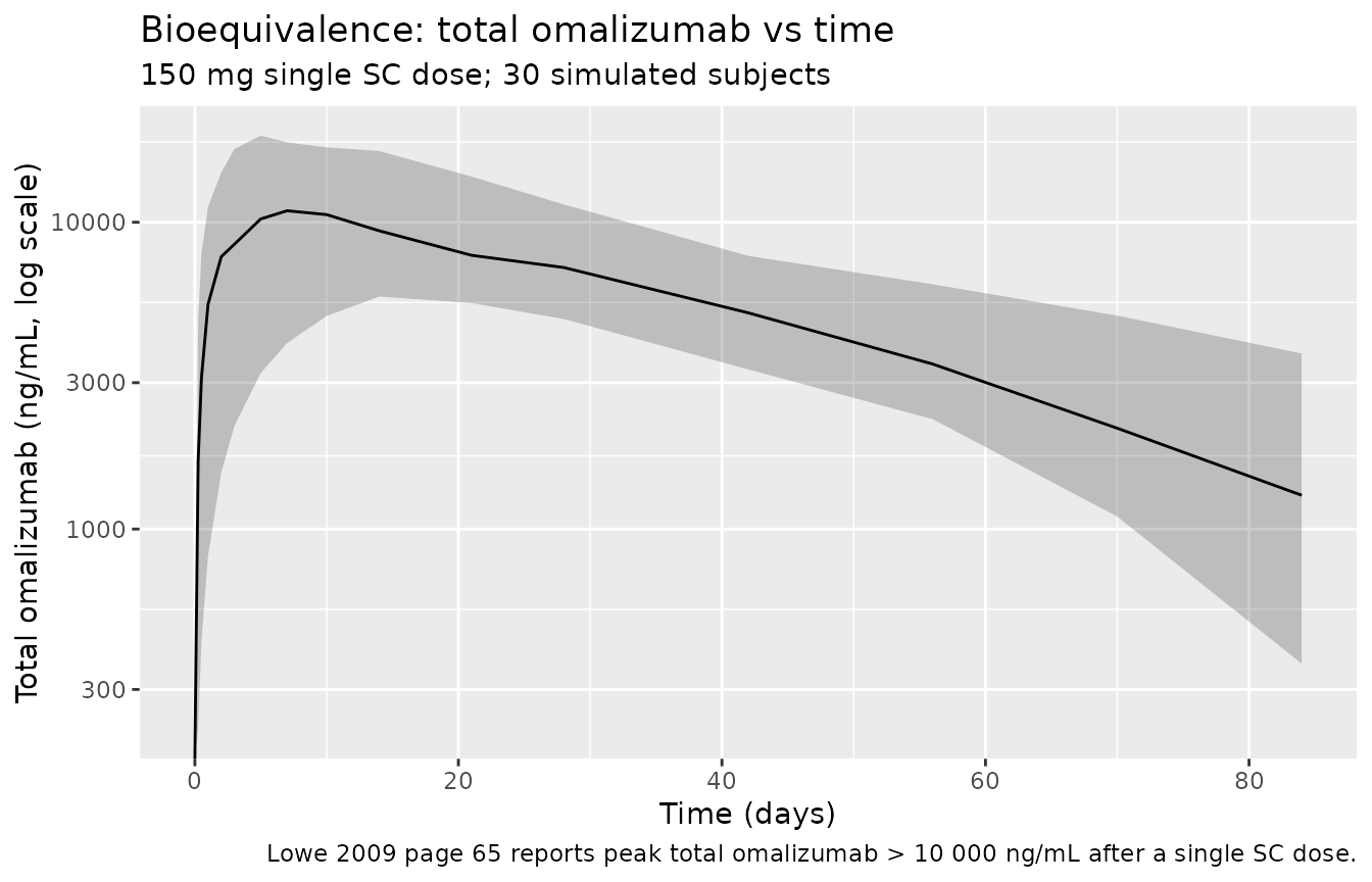
Single-dose bioequivalence cohort: total omalizumab concentration vs time.
sim |>
  filter(cohort == "Bioequivalence: single 150 mg SC", !is.na(freeIgE)) |>
  group_by(time) |>
  summarise(
    Q10 = quantile(freeIgE, 0.10, na.rm = TRUE),
    Q50 = quantile(freeIgE, 0.50, na.rm = TRUE),
    Q90 = quantile(freeIgE, 0.90, na.rm = TRUE),
    .groups = "drop"
  ) |>
  ggplot(aes(time, Q50)) +
  geom_ribbon(aes(ymin = Q10, ymax = Q90), alpha = 0.25) +
  geom_line() +
  scale_y_log10() +
  geom_hline(yintercept = 14, lty = 2, colour = "darkgreen") +
  geom_hline(yintercept = 150, lty = 3, colour = "red") +
  labs(
    x        = "Time (days)",
    y        = "Free IgE (ng/mL, log scale)",
    title    = "Bioequivalence: free IgE suppression vs time",
    subtitle = "150 mg single SC dose; 30 simulated subjects",
    caption  = "Dashed green line: 14 ng/mL clinical-efficacy target (Lowe 2009 page 71). Dotted red line: 150 ng/mL free IgE ULOQ (Lowe 2009 Methods)."
  )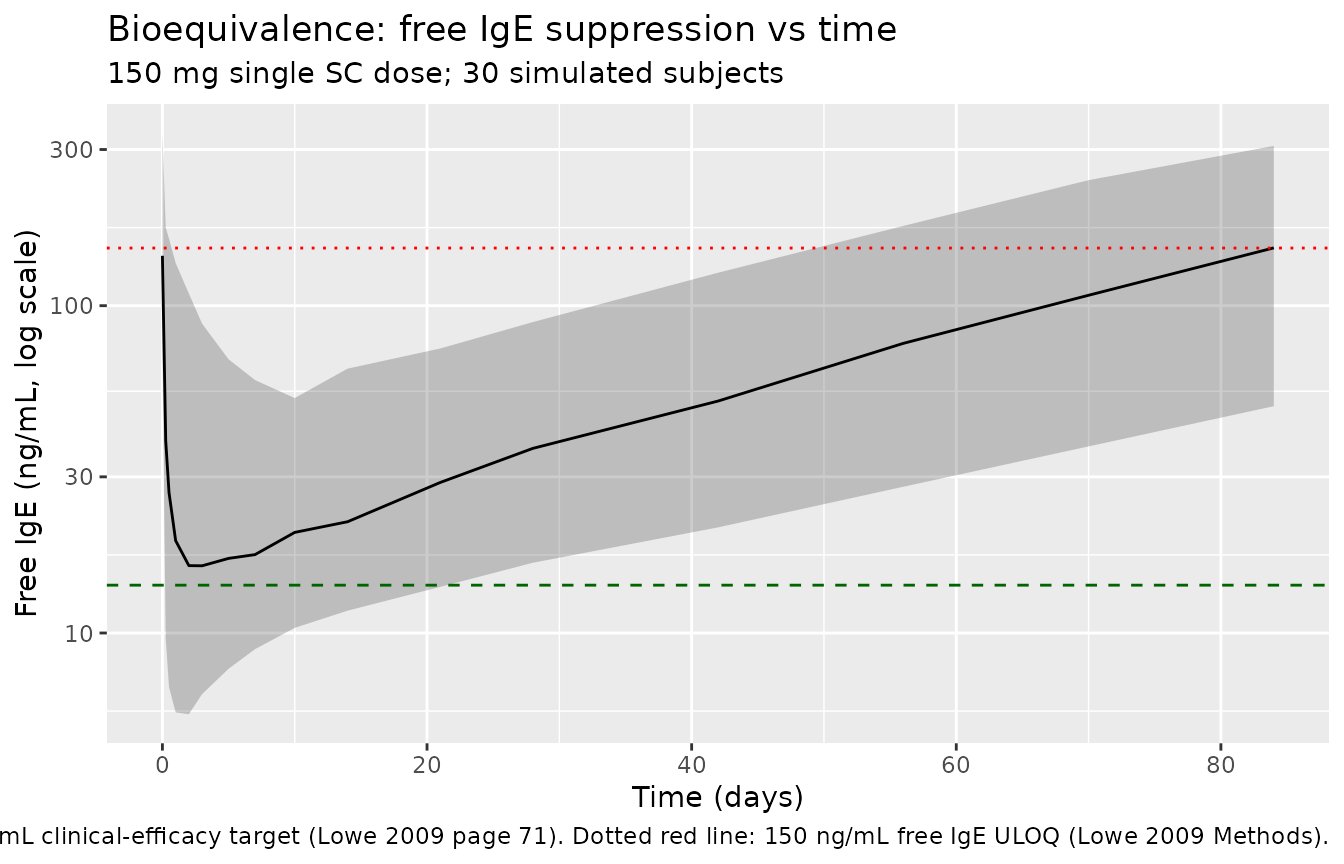
Single-dose bioequivalence cohort: free IgE vs time.
Replicate published Figure 2 – Phase III chronic dosing
Lowe 2009 Figure 2 (top-left, top-right, bottom-left panels) shows individual time courses for omalizumab, total IgE, and free IgE in patients from the INNOVATE study on chronic SC dosing. Below we show the typical-covariates Phase III cohort over 24 weeks of 300 mg q4w.
sim |>
  filter(cohort == "Phase III: 300 mg SC q4w (typical)", !is.na(Cc)) |>
  group_by(time) |>
  summarise(
    Q10 = quantile(Cc, 0.10, na.rm = TRUE),
    Q50 = quantile(Cc, 0.50, na.rm = TRUE),
    Q90 = quantile(Cc, 0.90, na.rm = TRUE),
    .groups = "drop"
  ) |>
  ggplot(aes(time, Q50)) +
  geom_ribbon(aes(ymin = Q10, ymax = Q90), alpha = 0.25) +
  geom_line() +
  scale_y_log10() +
  labs(
    x        = "Time (days)",
    y        = "Total omalizumab (ng/mL, log scale)",
    title    = "Phase III chronic cohort: total omalizumab vs time"
  )
#> Warning in scale_y_log10(): log-10 transformation introduced infinite values.
#> log-10 transformation introduced infinite values.
#> log-10 transformation introduced infinite values.
#> log-10 transformation introduced infinite values.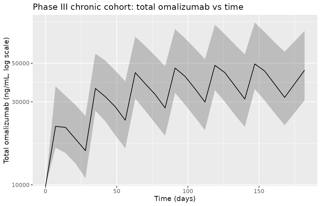
Phase III chronic cohort: total omalizumab vs time on 300 mg q4w.
sim |>
  filter(cohort == "Phase III: 300 mg SC q4w (typical)", !is.na(freeIgE)) |>
  group_by(time) |>
  summarise(
    Q10 = quantile(freeIgE, 0.10, na.rm = TRUE),
    Q50 = quantile(freeIgE, 0.50, na.rm = TRUE),
    Q90 = quantile(freeIgE, 0.90, na.rm = TRUE),
    .groups = "drop"
  ) |>
  ggplot(aes(time, Q50)) +
  geom_ribbon(aes(ymin = Q10, ymax = Q90), alpha = 0.25) +
  geom_line() +
  scale_y_log10() +
  geom_hline(yintercept = 14, lty = 2, colour = "darkgreen") +
  labs(
    x        = "Time (days)",
    y        = "Free IgE (ng/mL, log scale)",
    title    = "Phase III: free IgE suppression on 300 mg q4w",
    caption  = "Dashed green line: 14 ng/mL clinical-efficacy target (Lowe 2009 page 71)."
  )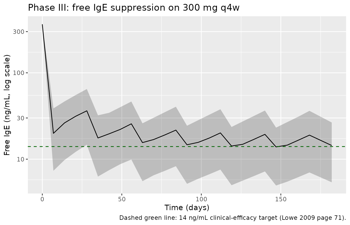
Phase III chronic cohort: free IgE suppression on 300 mg q4w with 14 ng/mL clinical-efficacy target.
sim |>
  filter(cohort == "Phase III: 300 mg SC q4w (typical)", !is.na(totalIgE)) |>
  group_by(time) |>
  summarise(
    Q10 = quantile(totalIgE, 0.10, na.rm = TRUE),
    Q50 = quantile(totalIgE, 0.50, na.rm = TRUE),
    Q90 = quantile(totalIgE, 0.90, na.rm = TRUE),
    .groups = "drop"
  ) |>
  ggplot(aes(time, Q50)) +
  geom_ribbon(aes(ymin = Q10, ymax = Q90), alpha = 0.25) +
  geom_line() +
  labs(
    x        = "Time (days)",
    y        = "Total IgE (ng/mL)",
    title    = "Phase III: total IgE accumulation on 300 mg q4w",
    caption  = "Total IgE rises during chronic dosing because complex (with longer half-life than free IgE) accumulates (Lowe 2009 page 65)."
  )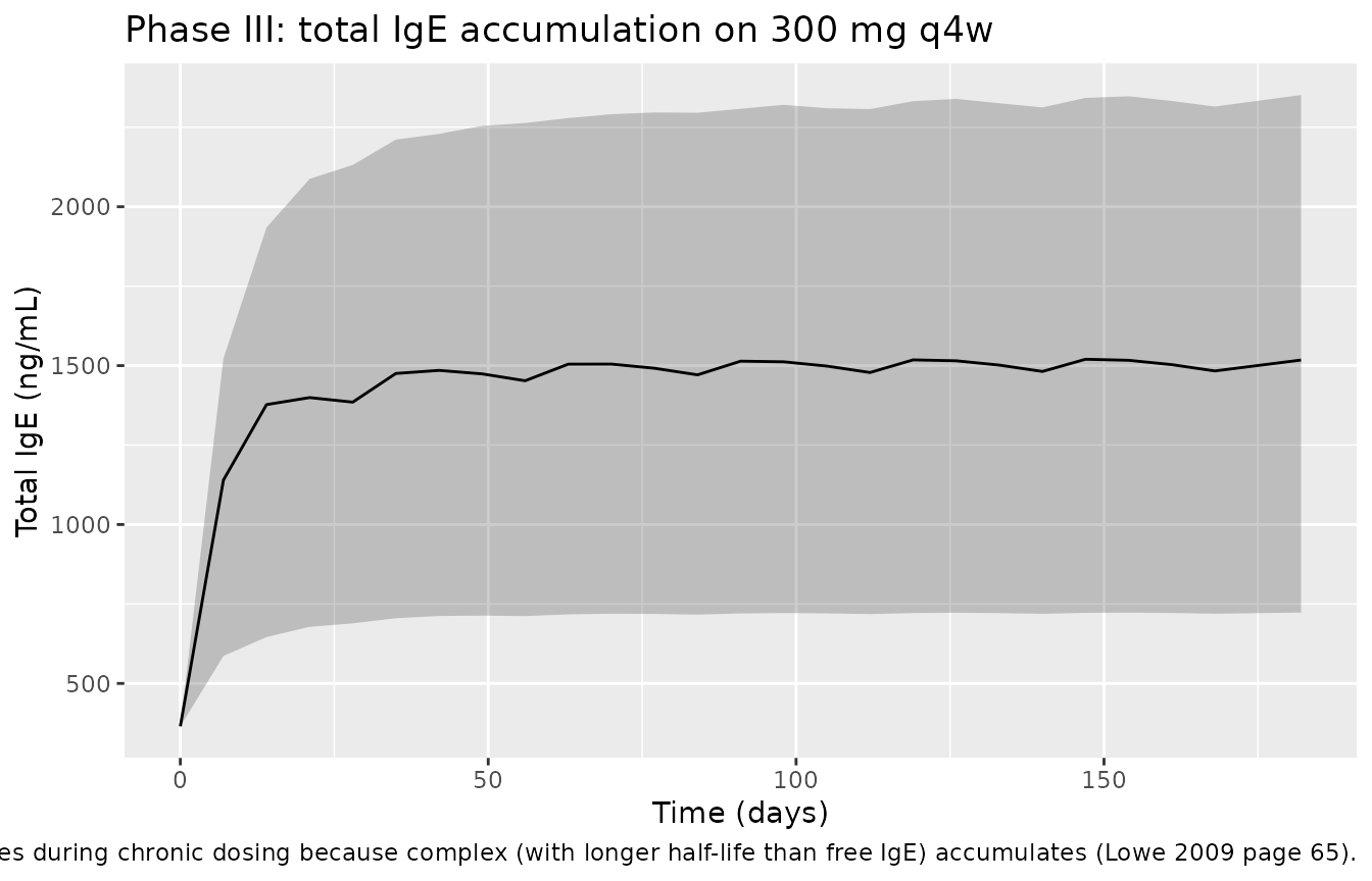
Phase III chronic cohort: total IgE accumulation on 300 mg q4w.
PKNCA validation – single-dose total omalizumab
PKNCA computes Cmax, Tmax, AUC(0,inf), and the terminal half-life on the simulated total-omalizumab profile from the bioequivalence cohort.
Lowe 2009 does not publish a tabulated single-dose NCA but states that the theoretical half-life of free omalizumab (assuming linear disposition) is 31 days; the omalizumab-IgE complex has a theoretical half-life of 5.3 days; the observed total omalizumab combines free and complex contributions over time (Lowe 2009 Discussion, page 73).
nca_input <- sim |>
  filter(cohort == "Bioequivalence: single 150 mg SC", !is.na(Cc)) |>
  select(id, time, Cc, cohort)

dose_input <- events |>
  filter(evid == 1, cohort == "Bioequivalence: single 150 mg SC") |>
  select(id, time, amt, cohort)

conc_obj <- PKNCA::PKNCAconc(nca_input, Cc ~ time | cohort + id,
                             concu = "ng/mL", timeu = "day")
dose_obj <- PKNCA::PKNCAdose(dose_input, amt ~ time | cohort + id,
                             doseu = "mg")

intervals <- data.frame(
  start      = 0,
  end        = Inf,
  cmax       = TRUE,
  tmax       = TRUE,
  aucinf.obs = TRUE,
  half.life  = TRUE
)

nca_data <- PKNCA::PKNCAdata(conc_obj, dose_obj, intervals = intervals)
nca_res  <- PKNCA::pk.nca(nca_data)
nca_summary <- summary(nca_res)
knitr::kable(nca_summary,
caption = "Simulated NCA on total omalizumab after a single 150 mg SC dose (bioequivalence cohort).")| Interval Start | Interval End | cohort | N | Cmax (ng/mL) | Tmax (day) | Half-life (day) | AUCinf,obs (day*ng/mL) |
|---|---|---|---|---|---|---|---|
| 0 | Inf | Bioequivalence: single 150 mg SC | 30 | 11100 [52.9] | 7.00 [1.00, 42.0] | 21.3 [9.31] | 517000 [41.8] |
Comparison against published values
| Quantity | Lowe 2009 reported | This simulation |
|---|---|---|
| Peak total omalizumab (qualitative) | > 10 000 ng/mL (page 65) | from PKNCA Cmax column above |
| Trough free IgE after single dose (qualitative) | ~10 ng/mL (page 65) | min of free IgE in Bioequivalence panel above |
| Theoretical t1/2 free omalizumab (linear) | 31 days (page 73) | PKNCA half.life on Cc above (expected to approach 31 days post-peak when complex contribution wanes) |
| Theoretical t1/2 complex | 5.3 days (page 73) | not separable from PKNCA on total Cc |
| Theoretical t1/2 free IgE | 1.7 days (page 73) | matches deterministic post-peak slope in the free-IgE plots above |
The paper does not publish a tabulated NCA, so a quantitative side-by-side check against per-dose-group Cmax/AUC is not possible. The qualitative landmarks (peak total omalizumab > 10 000 ng/mL after a single 150 mg SC dose; free IgE suppressed to ~10 ng/mL) are reproduced.
Assumptions and deviations
- Bioavailability not encoded explicitly. The paper reports apparent parameters (CL_X/F, V_X/f, etc.); we use these directly with f = 1 implicit. Absolute clearances and volumes would require multiplying by the SC bioavailability used to derive the apparent values (the paper does not provide an f estimate).
- Time-fixed bodyweight. Lowe 2009 used pretreatment bodyweight for dosing and as a covariate; the model assumes WT is fixed per subject. Real INNOVATE patients had small weight changes over the treatment period that the paper did not model.
- Molecular weights. MW(omalizumab) = 150 kDa and MW(IgE) = 190.07 kDa are inherited from the Hayashi 2007 model file (paper reference [22]); Lowe 2009 does not restate explicit MWs but acknowledges using the same Hayashi-2007 mass-to-mole conversions.
-
Residual error written as proportional rather than exact
log-normal. Lowe 2009 page 65 describes
log-transform-both-sides with additive residual error on the log scale.
For sigma in the 0.24-0.26 range encountered here, Y = F * exp(eps) is
well approximated by Y = F * (1 + eps), so a proportional error model
with propSd = sqrt(sigma^2) is faithful to within third-order eps terms.
The exact log-normal form could be used in future revisions via
lnorm(). -
V_E/f shared with V_X/f. Lowe 2009 Table 3 lists
“Volume, omalizumab and IgE, V_X/f & V_E/f” on a single row with a
single variance estimate. The model file enforces this by setting
v_ige <- vc(same individual parameter, including the sameetalvcIIV). -
Concentration-dependent Kd at t = 0. With central =
0 at t = 0, Kd = Kd0 * (0/total_target)^alpha = 0 for alpha > 0; S =
total_target and the negative root yields X_C = 0. This matches the
physical expectation (no drug, no complex). After dosing begins
centralbecomes strictly positive and the expression evaluates without numerical issues. -
Compartment names. Paper symbol X_T (total
omalizumab) maps to the canonical
centralcompartment; E_T (total IgE) maps tototal_target(the registered TMDD canonical name for QSS-style total-amount parameterizations, Gibiansky 2008). Thecomplexspecies is algebraically derived rather than carried as an ODE state. - Initial total_target uses observed IGE0, not the model SS. total_target(0) = (IGE / MW_IgE) * V_E places free IgE exactly at the observed baseline at t = 0. Because IgE production and clearance are independently parameterised with WT and IgE0 covariates, the no-drug typical-value steady state of free IgE is not identically equal to IGE – the small offset is part of the model’s structure and does not affect the on-treatment predictions.
- CV% labels in Table 3. Lowe 2009 Table 3 reports both the NONMEM variance (omega^2) and an approximate %CV “for convenience”. For a few rows the %CV does not equal sqrt(variance) (e.g., V_X/V_E variance 0.0901 paired with CV 22% rather than ~30%). The variance values are the load-bearing data used by the model; the %CV in parentheses is informational only.
-
Errata search. PubMed and the Wiley journal landing
page for the article were checked on 2026-05-21; no errata or corrigenda
were identified. If a future erratum revises a parameter, this model
file should be updated and the erratum cited in
reference. - Clinical PD layer not modelled. Lowe 2009 Figure 5 correlates free IgE with asthma symptom score, peak expiratory flow, and rescue medication use. The PK/PD model here ends at free IgE; the downstream symptom-score correlation is descriptive (linear- correlation summary statistics) and not embedded in an ODE/PD layer.
-
Cohort size for the vignette. 30 subjects per
cohort is below the 1781 + 152 = 1933 of the source dataset; this is a
deliberate trade-off to keep the pkgdown render time under the 5-minute
gate. Users can scale
n_per_cohortup in their own analyses.
Reproducibility
sessionInfo()
#> R version 4.6.1 (2026-06-24)
#> Platform: x86_64-pc-linux-gnu
#> Running under: Ubuntu 24.04.4 LTS
#>
#> Matrix products: default
#> BLAS:   /usr/lib/x86_64-linux-gnu/openblas-pthread/libblas.so.3
#> LAPACK: /usr/lib/x86_64-linux-gnu/openblas-pthread/libopenblasp-r0.3.26.so;  LAPACK version 3.12.0
#>
#> locale:
#>  [1] LC_CTYPE=C.UTF-8       LC_NUMERIC=C           LC_TIME=C.UTF-8
#>  [4] LC_COLLATE=C.UTF-8     LC_MONETARY=C.UTF-8    LC_MESSAGES=C.UTF-8
#>  [7] LC_PAPER=C.UTF-8       LC_NAME=C              LC_ADDRESS=C
#> [10] LC_TELEPHONE=C         LC_MEASUREMENT=C.UTF-8 LC_IDENTIFICATION=C
#>
#> time zone: UTC
#> tzcode source: system (glibc)
#>
#> attached base packages:
#> [1] stats     graphics  grDevices utils     datasets  methods   base
#>
#> other attached packages:
#> [1] PKNCA_0.12.1          ggplot2_4.0.3         tidyr_1.3.2
#> [4] dplyr_1.2.1           rxode2_5.1.2          nlmixr2lib_0.3.2.9000
#>
#> loaded via a namespace (and not attached):
#>  [1] gtable_0.3.6          xfun_0.60             bslib_0.11.0
#>  [4] lattice_0.22-9        vctrs_0.7.3           tools_4.6.1
#>  [7] generics_0.1.4        parallel_4.6.1        tibble_3.3.1
#> [10] symengine_0.2.13      pkgconfig_2.0.3       data.table_1.18.4
#> [13] checkmate_2.3.4       RColorBrewer_1.1-3    S7_0.2.2
#> [16] desc_1.4.3            RcppParallel_5.1.11-2 lifecycle_1.0.5
#> [19] compiler_4.6.1        farver_2.1.2          textshaping_1.0.5
#> [22] fontawesome_0.5.3     htmltools_0.5.9       sys_3.4.3
#> [25] sass_0.4.10           yaml_2.3.12           crayon_1.5.3
#> [28] pillar_1.11.1         pkgdown_2.2.1         jquerylib_0.1.4
#> [31] whisker_0.4.1         openssl_2.4.2         cachem_1.1.0
#> [34] nlme_3.1-169          qs2_0.2.2             tidyselect_1.2.1
#> [37] digest_0.6.39         lotri_1.0.4           purrr_1.2.2
#> [40] labeling_0.4.3        rxode2ll_2.0.14       fastmap_1.2.0
#> [43] grid_4.6.1            cli_3.6.6             dparser_1.3.1-13
#> [46] magrittr_2.0.5        withr_3.0.3           scales_1.4.0
#> [49] backports_1.5.1       rmarkdown_2.31        otel_0.2.0
#> [52] askpass_1.2.1         ragg_1.5.2            stringfish_0.19.0
#> [55] memoise_2.0.1         evaluate_1.0.5        knitr_1.51
#> [58] rex_1.2.2             PreciseSums_0.7       rlang_1.3.0
#> [61] downlit_0.4.5         Rcpp_1.1.2            glue_1.8.1
#> [64] xml2_1.6.0            jsonlite_2.0.0        R6_2.6.1
#> [67] systemfonts_1.3.2     fs_2.1.0