Pegcetacoplan intravitreal (Crass 2025)
Source:vignettes/articles/Crass_2025_pegcetacoplan_intravitreal.Rmd
Crass_2025_pegcetacoplan_intravitreal.RmdModel and source
mod_name <- "Crass_2025_pegcetacoplan_intravitreal"
ui <- rxode2::rxode(readModelDb(mod_name))
#> ℹ parameter labels from comments will be replaced by 'label()'- Citation: Crass RL, Prem K, Gaudreault F, Ribeiro R, Baumal CR, Smith B, Epling D, Chapel S. Population Pharmacokinetics of Pegcetacoplan in Patients with Geographic Atrophy or Neovascular Age-related Macular Degeneration. Ophthalmol Sci. 2025;5(2):100657. doi:10.1016/j.xops.2024.100657
- Description: One-compartment population PK model for serum pegcetacoplan after intravitreal injection in adults with geographic atrophy or neovascular age-related macular degeneration (Crass 2025). The intravitreal dose enters a vitreous compartment and is absorbed into the systemic (serum) central compartment by a first-order rate ka that is slower than systemic elimination (flip-flop kinetics); systemic bioavailability is assumed to be 1, so CL and Vc are the apparent values CL/F and Vc/F. CL/F carries power effects of age (reference 80 years) and baseline serum complement C3 (reference 1.2 g/L) and a log-linear female-sex effect. Inter-individual variability is on CL/F (Manly / Box-Cox transformed eta) and ka; Vc/F has no random effect. Residual error is additive on the log scale (log-normal). Vitreous concentration is derived from the vitreous amount over an assumed 4 mL vitreous volume and is not observed.
- Article: Ophthalmol Sci 2025;5(2):100657
Pegcetacoplan is a pegylated peptide inhibitor of complement C3
approved for geographic atrophy (GA) secondary to age-related macular
degeneration. It is injected into the vitreous, and only serum
concentrations can be measured, so the authors fitted a population PK
model to serum data and used it to infer the vitreous exposure. The
vitreous concentration predicted by this model is the exposure that
drives the GA lesion-growth exposure-response model of the companion
paper, Crass_2025_pegcetacoplan_ga_exposureresponse (see
the Crass
2025 GA lesion-area article), which supplies it as the
CEFFECT covariate.
Population
The analysis pooled 2064 serum samples from 261 patients in four studies: POT-CP043014 (n = 13) and APL2-203 (n = 17) in neovascular AMD (nAMD), and POT-CP121614 / FILLY (n = 164) and APL2-303 / DERBY (n = 67) in GA. Doses were single intravitreal injections of 4, 10 or 20 mg and repeated 15 mg injections monthly or every other month. Mean (SD) age was 79.6 (7.69) years, 56.7% were female, 97.3% were White, and mean (SD) baseline serum C3 was 1.20 (0.241) g/L. 88.5% had GA, and 73.9% had mild or moderate renal impairment (Crass 2025 Table 1). 23.4% of samples were below the 0.10 ug/mL lower limit of quantification and were handled with the M3 likelihood method.
The same information is available programmatically:
str(ui$population)
#> List of 13
#>  $ species       : chr "human"
#>  $ n_subjects    : int 261
#>  $ n_studies     : int 4
#>  $ n_observations: int 2064
#>  $ age_mean      : chr "79.6 years (SD 7.69)"
#>  $ sex_female_pct: num 56.7
#>  $ race_ethnicity: Named num [1:3] 97.3 0.8 1.9
#>   ..- attr(*, "names")= chr [1:3] "White" "Black" "Other_or_missing"
#>  $ disease_state : chr "Geographic atrophy secondary to age-related macular degeneration (n = 231, 88.5%) or neovascular age-related ma"| __truncated__
#>  $ dose_range    : chr "Single intravitreal injections of 4, 10 or 20 mg, and repeated intravitreal injections of 15 mg monthly or every other month."
#>  $ renal_function: chr "Normal 19.5%, mild impairment 42.9%, moderate 31.0%, severe 0.8%, end stage 4.2% (Table 1)."
#>  $ c3_mean       : chr "1.20 g/L (SD 0.241)"
#>  $ studies       : chr "POT-CP043014 (n = 13, nAMD), APL2-203 (n = 17, nAMD), POT-CP121614 / FILLY (n = 164, GA), APL2-303 / DERBY (n = 67, GA)."
#>  $ notes         : chr "Serum PK only; 1581 of 2064 samples (76.6%) were quantifiable and 483 (23.4%) were below the 0.10 ug/mL lower l"| __truncated__
Source trace
Every ini() value carries an in-file comment naming its
source. The table collects them. Table 2 of the paper prints the
log-scale NONMEM estimates alongside their exponentials; the minus signs
of the log-scale column are present in the PDF as a separate glyph that
some text extractors drop, and the direction of every Figure 2
forest-plot ratio confirms them (see the forest-plot replication
below).
| Equation / parameter | Value | Source location |
|---|---|---|
lka (ka) |
log(0.0528) 1/day | Table 2, KA estimate -2.94, transformed 0.0528 |
lcl (CL/F) |
log(0.325) L/day | Table 2, CL/F estimate -1.12, transformed 0.325 |
lvc (Vc/F) |
log(1.83) L | Table 2, VC/F estimate 0.603, transformed 1.83 |
e_age_cl |
-0.559 | Table 2, ‘Age on CL/F (theta6)’ |
e_c3_bl_cl |
-0.350 | Table 2, ‘C3 on CL/F (theta7)’ |
e_sexf_cl |
-0.286 (0.751-fold) | Table 2, ‘Female sex on CL/F (theta8)’ |
boxcox_lcl |
2.57 | Table 2, ‘Lambda’ |
etalcl |
0.0587 | Table 2, IIV omega^2 CL/F |
etalka |
0.122 (36.0% CV) | Table 2, IIV omega^2 KA |
expSd |
0.300 | Table 2, residual variability, log additive |
covcl = theta6 log(Age/80) + theta7 log(C3/1.2) +
theta8 FemaleSex |
n/a | Table 2 footnote equation COVCL |
etatrcl = (exp(eta lambda) - 1) / lambda |
n/a | Table 2 footnote equation TETACL (Manly transformation, Methods) |
cl = exp(lcl + covcl + etatrcl); vc =
exp(lvc); ka = exp(lka + etalka) |
n/a | Table 2 footnote equations |
d/dt(vitreous), d/dt(central)
|
n/a | Figure 1; Methods, Model Development |
| Systemic bioavailability = 1 | n/a | Methods, Model Development |
Vitreous volume 4 mL in Cvit
|
n/a | Methods, Model Development |
Cc ~ lnorm(expSd) |
n/a | Methods, Model Parameterization (log-transform-both-sides) |
The Manly transform written in Table 2,
(exp(eta * lambda) - 1) / lambda, is identical to the
Box-Cox form (exp(eta)^lambda - 1) / lambda, which is why
the shape parameter carries the library’s boxcox_ name.
Typical-value checks
The model is linear, so the typical patient (male, 80 years, C3 1.2 g/L) has closed-form serum and vitreous concentrations. These gates compare the ODE solve with the closed form at tight tolerances.
typ <- rxode2::zeroRe(ui)
ka <- exp(ui$theta[["lka"]])
cl <- exp(ui$theta[["lcl"]])
vc <- exp(ui$theta[["lvc"]])
kel <- cl / vc
dose <- 15

ev_typ <- data.frame(
  id = 1L,
  time = c(0, seq(0.25, 120, by = 0.25)),
  evid = c(1L, rep(0L, 480)),
  amt = c(dose, rep(NA_real_, 480)),
  cmt = "vitreous",
  AGE = 80, C3_BL = 1.2, SEXF = 0
)
sim_typ <- as.data.frame(rxode2::rxSolve(typ, ev_typ, rtol = 1e-10, atol = 1e-12))
#> ℹ omega/sigma items treated as zero: 'etalcl', 'etalka'
obs_typ <- sim_typ[sim_typ$time > 0, ]
cvit_cf <- dose / 4 * 1000 * exp(-ka * obs_typ$time)
cc_cf <- dose * ka / (vc * (ka - kel)) * (exp(-kel * obs_typ$time) - exp(-ka * obs_typ$time))
err_vit <- max(abs(obs_typ$Cvit / cvit_cf - 1))
err_cc <- max(abs(obs_typ$Cc / cc_cf - 1))

half_lives <- data.frame(
  Quantity = c("Absorption half-life ln(2)/ka (days)", "Elimination half-life ln(2)*Vc/CL (days)"),
  Model = c(log(2) / ka, log(2) / kel),
  Paper = c("13.1 (geometric mean)", "4.51 (median of empirical Bayes estimates)")
)
knitr::kable(half_lives, digits = 2)| Quantity | Model | Paper |
|---|---|---|
| Absorption half-life ln(2)/ka (days) | 13.13 | 13.1 (geometric mean) |
| Elimination half-life ln(2)*Vc/CL (days) | 3.90 | 4.51 (median of empirical Bayes estimates) |
stopifnot(
  err_vit < 1e-6,
  err_cc < 1e-6,
  # Results: geometric-mean absorption half-life 13.1 days. The geometric mean
  # of ka is its typical value, so this is a deterministic identity.
  abs(log(2) / ka - 13.1) < 0.05
)

# Values quoted in Assumptions and deviations to explain two Table 3 entries:
# the serum concentration half a day after injection, and the vitreous
# concentration left at the end of a 30- and a 60-day interval.
cc_half_day <- sim_typ$Cc[sim_typ$time == 0.5]
cvit_end <- dose / 4 * 1000 * exp(-ka * c(30, 60))
stopifnot(
  length(cc_half_day) == 1L,
  abs(cc_half_day - 0.204) < 0.001,
  abs(cvit_end[1] - 769) < 1,
  abs(cvit_end[2] - 158) < 1,
  # Table 3 first-dose vitreous Cmax medians 4523 and 3903 ug/mL
  abs((3750 + cvit_end[1]) / 4523 - 1) < 0.01,
  abs((3750 + cvit_end[2]) / 3903 - 1) < 0.01
)
The absorption half-life reproduces the reported 13.1 days. The reported 4.51-day elimination half-life is a median over the analysis population, not a typical-value quantity. The typical patient is male, and the female CL/F of 0.751-fold gives a 5.20-day half-life, so a population median between the male (3.90 days) and female values is expected.
sim_typ |>
  dplyr::select(time, `Serum (ug/mL)` = Cc, `Vitreous (ug/mL)` = Cvit) |>
  tidyr::pivot_longer(-time, names_to = "matrix", values_to = "conc") |>
  dplyr::filter(conc > 0) |>
  ggplot(aes(time, conc)) +
  geom_line() +
  facet_wrap(~matrix, scales = "free_y") +
  scale_y_log10() +
  labs(x = "Time after injection (days)", y = "Pegcetacoplan concentration (ug/mL)")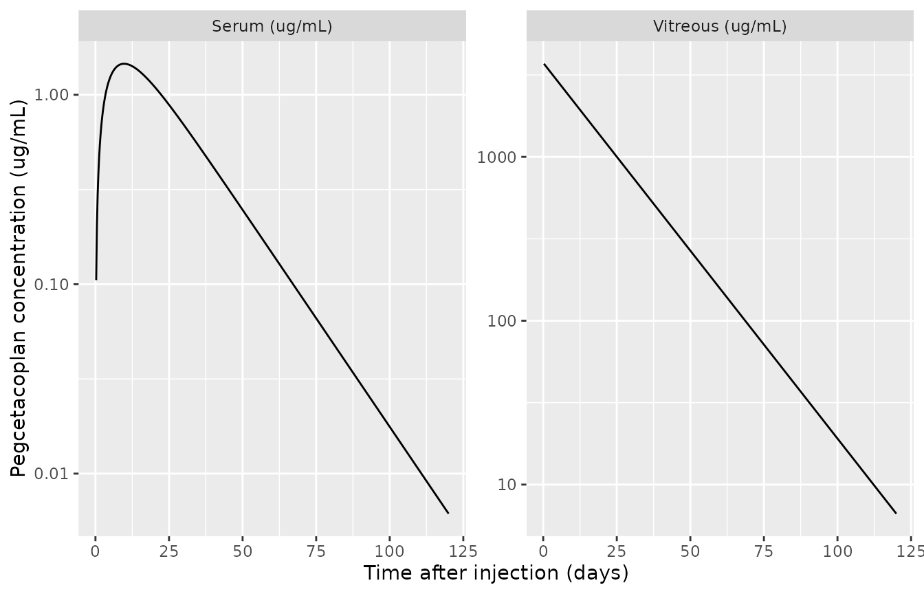
Typical-patient serum and vitreous concentrations after a single 15 mg intravitreal injection.
Replicate Figure 2 (covariate forest plot)
Figure 2 shows the steady-state serum AUC, Cmax and Cmin of a patient who differs from the reference (male, 80 years, C3 1.2 g/L) in one covariate, for 15 mg monthly. The ratios are medians over 1000 bootstrap parameter sets, so they match the point-estimate model when the bootstrap is centred. Monthly dosing is taken as every 30 days, the interval implied by Table 3, where vitreous AUC divided by Cavg is 30.0 days.
ss_metrics <- function(AGE = 80, C3_BL = 1.2, SEXF = 0, tau = 30, n_dose = 40) {
  dose_times <- seq(0, (n_dose - 1) * tau, by = tau)
  obs_times <- seq((n_dose - 1) * tau, n_dose * tau, by = 0.05)
  ev <- data.frame(
    id = 1L,
    time = c(dose_times, obs_times),
    evid = c(rep(1L, length(dose_times)), rep(0L, length(obs_times))),
    amt = c(rep(dose, length(dose_times)), rep(NA_real_, length(obs_times))),
    cmt = "vitreous",
    AGE = AGE, C3_BL = C3_BL, SEXF = SEXF
  )
  r <- as.data.frame(rxode2::rxSolve(typ, ev, rtol = 1e-10, atol = 1e-12, maxsteps = 1e6))
  # Drop the post-dose row at the interval end so the interval is [t, t + tau).
  r <- r[r$time < n_dose * tau, ]
  c(
    auc = sum(diff(r$time) * (head(r$Cc, -1) + tail(r$Cc, -1)) / 2),
    cmax = max(r$Cc),
    cmin = min(r$Cc)
  )
}

ref_ss <- ss_metrics()
#> ℹ omega/sigma items treated as zero: 'etalcl', 'etalka'
scenarios <- tibble::tribble(
  ~covariate, ~AGE, ~C3_BL, ~SEXF, ~auc_pub, ~cmax_pub, ~cmin_pub,
  "Sex (Female : Male)", 80, 1.2, 1, 1.33, 1.26, 1.46,
  "Age (92 : 80 years)", 92, 1.2, 0, 1.08, 1.07, 1.11,
  "Age (68 : 80 years)", 68, 1.2, 0, 0.914, 0.929, 0.888,
  "C3 (1.62 : 1.2 g/L)", 80, 1.62, 0, 1.11, 1.09, 1.15,
  "C3 (0.83 : 1.2 g/L)", 80, 0.83, 0, 0.879, 0.900, 0.844
)
forest <- scenarios |>
  dplyr::rowwise() |>
  dplyr::mutate(
    m = list(ss_metrics(AGE = AGE, C3_BL = C3_BL, SEXF = SEXF) / ref_ss),
    auc_sim = m[["auc"]],
    cmax_sim = m[["cmax"]],
    cmin_sim = m[["cmin"]]
  ) |>
  dplyr::ungroup() |>
  dplyr::select(covariate, auc_pub, auc_sim, cmax_pub, cmax_sim, cmin_pub, cmin_sim)
#> ℹ omega/sigma items treated as zero: 'etalcl', 'etalka'
#> ℹ omega/sigma items treated as zero: 'etalcl', 'etalka'
#> ℹ omega/sigma items treated as zero: 'etalcl', 'etalka'
#> ℹ omega/sigma items treated as zero: 'etalcl', 'etalka'
#> ℹ omega/sigma items treated as zero: 'etalcl', 'etalka'

forest |>
  dplyr::rename(
    "Covariate (test : reference)" = covariate,
    "AUC ratio, Figure 2A" = auc_pub,
    "AUC ratio, model" = auc_sim,
    "Cmax ratio, Figure 2B" = cmax_pub,
    "Cmax ratio, model" = cmax_sim,
    "Cmin ratio, Figure 2C" = cmin_pub,
    "Cmin ratio, model" = cmin_sim
  ) |>
knitr::kable(digits = 3, caption = "Replicates Figure 2 of Crass 2025: steady-state serum exposure ratios relative to the reference patient.")| Covariate (test : reference) | AUC ratio, Figure 2A | AUC ratio, model | Cmax ratio, Figure 2B | Cmax ratio, model | Cmin ratio, Figure 2C | Cmin ratio, model |
|---|---|---|---|---|---|---|
| Sex (Female : Male) | 1.330 | 1.331 | 1.260 | 1.265 | 1.460 | 1.464 |
| Age (92 : 80 years) | 1.080 | 1.081 | 1.070 | 1.066 | 1.110 | 1.109 |
| Age (68 : 80 years) | 0.914 | 0.913 | 0.929 | 0.929 | 0.888 | 0.888 |
| C3 (1.62 : 1.2 g/L) | 1.110 | 1.111 | 1.090 | 1.090 | 1.150 | 1.149 |
| C3 (0.83 : 1.2 g/L) | 0.879 | 0.879 | 0.900 | 0.900 | 0.844 | 0.845 |
# Deterministic: every ratio is a function of the point estimates only. The
# largest deviation is printed rounding (0.005 on a 3-significant-figure
# value); a sign error on any Table 2 covariate coefficient moves its ratio
# by at least 10%.
stopifnot(
  max(abs(forest$auc_sim / forest$auc_pub - 1)) < 0.006,
  max(abs(forest$cmax_sim / forest$cmax_pub - 1)) < 0.006,
  max(abs(forest$cmin_sim / forest$cmin_pub - 1)) < 0.006,
  # Steady-state AUC over a dosing interval equals Dose / CL.
  abs(ref_ss[["auc"]] / (dose / cl) - 1) < 1e-3
)
forest |>
  tidyr::pivot_longer(-covariate, names_to = c("metric", "source"), names_sep = "_") |>
  dplyr::mutate(
    metric = factor(toupper(metric), levels = c("AUC", "CMAX", "CMIN"), labels = c("AUC", "Cmax", "Cmin")),
    source = ifelse(source == "pub", "Figure 2", "Model")
  ) |>
  ggplot(aes(value, covariate, shape = source)) +
  annotate("rect", xmin = 0.8, xmax = 1.25, ymin = -Inf, ymax = Inf, alpha = 0.15) +
  geom_vline(xintercept = 1, linetype = 2) +
  geom_point(size = 2.5) +
  scale_shape_manual(values = c("Figure 2" = 4, "Model" = 16)) +
  facet_wrap(~metric, ncol = 1) +
  labs(x = "Steady-state ratio relative to reference", y = NULL, shape = NULL)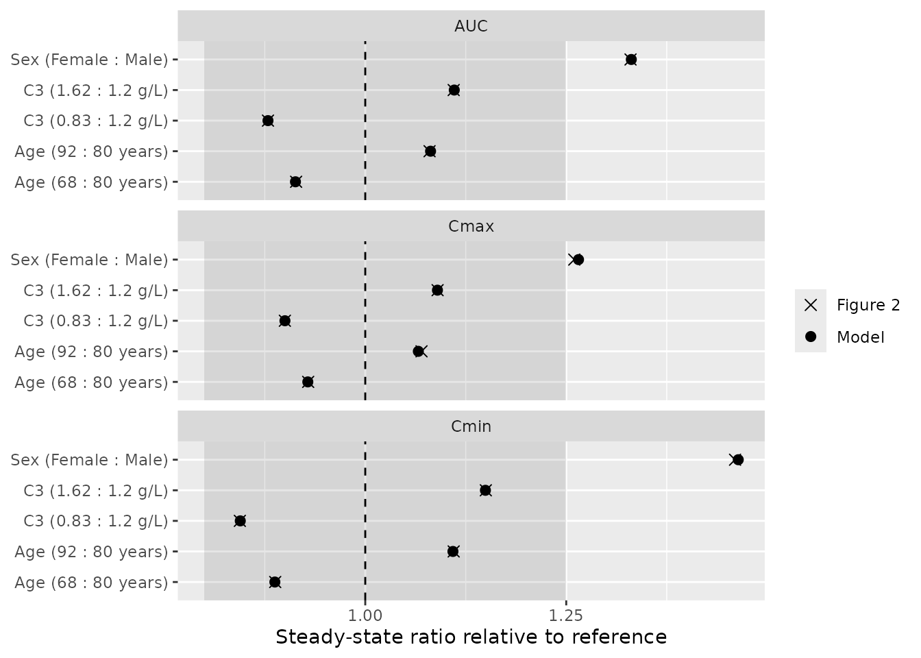
Replicates Figure 2 of Crass 2025 (points: model; crosses: published medians).
Virtual cohort
Table 3 of the paper summarises exposure in 121 GA patients given 15 mg monthly and 110 given 15 mg every other month. The individual covariates are not published, so the cohort below draws them from the GA studies of Table 1 (FILLY and DERBY, n = 231): age from a normal distribution with the pooled mean and SD (80.0 and 7.5 years), baseline C3 from a normal distribution with the pooled mean and SD (1.17 and 0.22 g/L), and 57.6% female. Draws outside 55 to 100 years or 0.5 to 2.2 g/L are redrawn rather than clamped.
set.seed(20250122)
rxode2::rxSetSeed(20250122)

draw_bounded <- function(n, mean, sd, lo, hi) {
  x <- rnorm(n, mean, sd)
  while (any(bad <- x < lo | x > hi)) {
    x[bad] <- rnorm(sum(bad), mean, sd)
  }
  x
}

n_per_arm <- 200L
regimens <- tibble::tribble(
  ~regimen, ~tau, ~n_dose,
  "15 mg monthly", 30, 12L,
  "15 mg every other month", 60, 6L
)
ss_start <- c("15 mg monthly" = 330, "15 mg every other month" = 300)

make_cohort <- function(regimen, tau, n_dose, id_offset) {
  subj <- tibble::tibble(
    id = id_offset + seq_len(n_per_arm),
    regimen = regimen,
    AGE = draw_bounded(n_per_arm, 80.0, 7.5, 55, 100),
    C3_BL = draw_bounded(n_per_arm, 1.17, 0.22, 0.5, 2.2),
    SEXF = rbinom(n_per_arm, 1, 0.576)
  )
  doses <- tidyr::crossing(subj, time = seq(0, (n_dose - 1) * tau, by = tau)) |>
    dplyr::mutate(evid = 1L, amt = dose)
  obs <- tidyr::crossing(subj, time = seq(0, 360, by = 0.5)) |>
    dplyr::mutate(evid = 0L, amt = NA_real_)
  dplyr::bind_rows(doses, obs) |>
    dplyr::mutate(cmt = "vitreous") |>
    dplyr::arrange(id, time, dplyr::desc(evid))
}

events <- dplyr::bind_rows(
  make_cohort(regimens$regimen[1], regimens$tau[1], regimens$n_dose[1], 0L),
  make_cohort(regimens$regimen[2], regimens$tau[2], regimens$n_dose[2], n_per_arm)
)
stopifnot(!anyDuplicated(unique(events[, c("id", "time", "evid")])))
Simulation
# `Cc` in the output is the individual prediction; the residual-error draw is
# in `sim` and is not used, because Table 3 summarises predicted exposure.
sim <- rxode2::rxSolve(
  ui,
  events = events,
  keep = c("regimen", "SEXF")
) |>
  as.data.frame() |>
  dplyr::mutate(regimen = as.character(regimen))
stopifnot(all(sim$Cc >= -1e-6 * max(sim$Cc)))
sim |>
  dplyr::select(regimen, time, `Serum (ug/mL)` = Cc, `Vitreous (ug/mL)` = Cvit) |>
  tidyr::pivot_longer(c(`Serum (ug/mL)`, `Vitreous (ug/mL)`), names_to = "matrix", values_to = "conc") |>
  dplyr::group_by(regimen, matrix, time) |>
  dplyr::summarise(
    Q05 = quantile(conc, 0.05),
    Q50 = median(conc),
    Q95 = quantile(conc, 0.95),
    .groups = "drop"
  ) |>
  ggplot(aes(time, Q50)) +
  geom_ribbon(aes(ymin = Q05, ymax = Q95), alpha = 0.25) +
  geom_line() +
  facet_grid(matrix ~ regimen, scales = "free_y") +
  labs(x = "Time (days)", y = "Pegcetacoplan concentration (ug/mL)")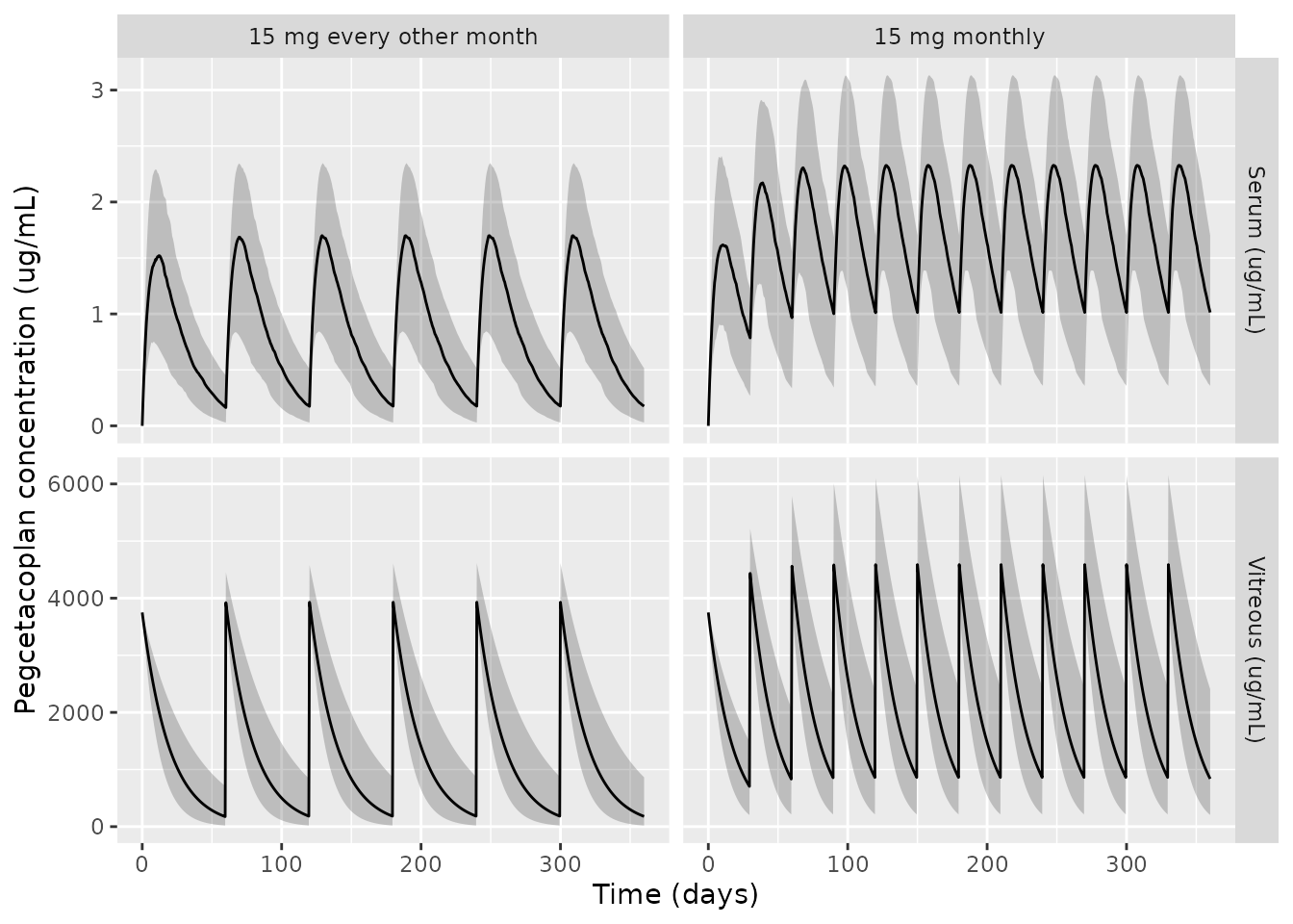
Simulated serum and vitreous pegcetacoplan over one year (median and 5th-95th percentile band, 200 patients per regimen).
PKNCA validation
Exposure metrics are computed over the first dosing interval and the steady-state interval (the 12th monthly or 6th every-other-month interval), separately for serum and vitreous. Concentrations are individual predictions without residual error.
nca_intervals <- dplyr::bind_rows(
  tibble::tibble(regimen = regimens$regimen, start = 0, end = regimens$tau),
  tibble::tibble(regimen = names(ss_start), start = unname(ss_start), end = unname(ss_start) + regimens$tau)
) |>
  dplyr::mutate(cmax = TRUE, cmin = TRUE, cav = TRUE, auclast = TRUE, tmax = TRUE)

dose_df <- events |>
  dplyr::filter(evid == 1) |>
  dplyr::select(id, time, amt, regimen)

run_nca <- function(conc_col) {
  conc_df <- sim |>
    dplyr::mutate(conc = .data[[conc_col]]) |>
    dplyr::filter(!is.na(conc)) |>
    dplyr::mutate(conc = pmax(conc, 0)) |>
    dplyr::select(id, time, conc, regimen)
  conc_obj <- PKNCA::PKNCAconc(conc_df, conc ~ time | regimen + id)
  dose_obj <- PKNCA::PKNCAdose(dose_df, amt ~ time | regimen + id)
  res <- PKNCA::pk.nca(PKNCA::PKNCAdata(conc_obj, dose_obj, intervals = nca_intervals))
  as.data.frame(res$result) |>
    dplyr::mutate(period = ifelse(start == 0, "First dose", "Steady state"))
}
nca_serum <- run_nca("Cc")
nca_vit <- run_nca("Cvit")
Comparison against published Table 3
Table 3 reports the median, the 5th and 95th percentiles, and the geometric mean of each metric. The comparison uses the medians. The first-dose serum Cmin is left out: over the first interval the serum minimum is the zero pre-dose value, and the published 0.200 / 0.100 ug/mL are the concentration at the first sampling point after the injection rather than a trough (see Assumptions and deviations).
pub_serum <- tibble::tribble(
  ~regimen, ~period, ~cmax, ~cmin, ~cav, ~auclast, ~tmax,
  "15 mg monthly", "First dose", 1.60, 0.200, 1.20, 35.9, 10.5,
  "15 mg monthly", "Steady state", 2.20, 1.10, 1.80, 52.8, 8.50,
  "15 mg every other month", "First dose", 1.50, 0.100, 0.800, 48.5, 10.2,
  "15 mg every other month", "Steady state", 1.70, 0.200, 0.900, 52.6, 10.0
)
pub_serum_long <- pub_serum |>
  tidyr::pivot_longer(c(cmax, cmin, cav, auclast, tmax), names_to = "PPTESTCD", values_to = "PPORRES") |>
  dplyr::filter(!(period == "First dose" & PPTESTCD == "cmin"))
nca_serum_cmp <- nca_serum |>
  dplyr::filter(!(period == "First dose" & PPTESTCD == "cmin"))
cmp_serum <- nlmixr2lib::ncaComparisonTable(
  simulated = nca_serum_cmp,
  reference = pub_serum_long,
  by = c("regimen", "period"),
  units = c(cmax = "ug/mL", cmin = "ug/mL", cav = "ug/mL", auclast = "ug*day/mL", tmax = "day"),
  tolerance_pct = 20
)
knitr::kable(cmp_serum, caption = "Serum: simulated vs. published (Table 3) medians. * differs by more than 20%.")| NCA parameter | regimen | period | Reference | Simulated | % diff |
|---|---|---|---|---|---|
| Cmax (ug/mL) | 15 mg monthly | First dose | 1.6 | 1.64 | +2.6% |
| Cmax (ug/mL) | 15 mg monthly | Steady state | 2.2 | 2.33 | +6.0% |
| Cmax (ug/mL) | 15 mg every other month | First dose | 1.5 | 1.55 | +3.3% |
| Cmax (ug/mL) | 15 mg every other month | Steady state | 1.7 | 1.71 | +0.7% |
| Cmin (ug/mL) | 15 mg monthly | Steady state | 1.1 | 1.01 | -7.9% |
| Cmin (ug/mL) | 15 mg every other month | Steady state | 0.2 | 0.176 | -12.1% |
| Tmax (day) | 15 mg monthly | First dose | 10.5 | 10 | -4.8% |
| Tmax (day) | 15 mg monthly | Steady state | 8.5 | 8.25 | -2.9% |
| Tmax (day) | 15 mg every other month | First dose | 10.2 | 10.5 | +2.9% |
| Tmax (day) | 15 mg every other month | Steady state | 10 | 10 | +0.0% |
| AUClast (ug*day/mL) | 15 mg monthly | First dose | 35.9 | 37.3 | +3.9% |
| AUClast (ug*day/mL) | 15 mg monthly | Steady state | 52.8 | 52.8 | -0.1% |
| AUClast (ug*day/mL) | 15 mg every other month | First dose | 48.5 | 46.7 | -3.6% |
| AUClast (ug*day/mL) | 15 mg every other month | Steady state | 52.6 | 51.5 | -2.1% |
| Cavg (ug/mL) | 15 mg monthly | First dose | 1.2 | 1.24 | +3.6% |
| Cavg (ug/mL) | 15 mg monthly | Steady state | 1.8 | 1.76 | -2.3% |
| Cavg (ug/mL) | 15 mg every other month | First dose | 0.8 | 0.779 | -2.6% |
| Cavg (ug/mL) | 15 mg every other month | Steady state | 0.9 | 0.859 | -4.6% |
pub_vit <- tibble::tribble(
  ~regimen, ~period, ~cmax, ~cmin, ~cav, ~auclast,
  "15 mg monthly", "First dose", 4523, 794, 1917, 57495,
  "15 mg monthly", "Steady state", 4724, 974, 2375, 71245,
  "15 mg every other month", "First dose", 3903, 157, 1139, 68353,
  "15 mg every other month", "Steady state", 3909, 159, 1171, 70275
)
cmp_vit <- nlmixr2lib::ncaComparisonTable(
  simulated = nca_vit,
  reference = pub_vit,
  by = c("regimen", "period"),
  params = c("cmax", "cmin", "cav", "auclast"),
  units = c(cmax = "ug/mL", cmin = "ug/mL", cav = "ug/mL", auclast = "ug*day/mL"),
  tolerance_pct = 20
)
knitr::kable(cmp_vit, caption = "Vitreous: simulated vs. published (Table 3) medians. * differs by more than 20%.")| NCA parameter | regimen | period | Reference | Simulated | % diff |
|---|---|---|---|---|---|
| Cmax (ug/mL) | 15 mg monthly | First dose | 4520 | 4430 | -2.0% |
| Cmax (ug/mL) | 15 mg monthly | Steady state | 4720 | 4590 | -2.9% |
| Cmax (ug/mL) | 15 mg every other month | First dose | 3900 | 3920 | +0.5% |
| Cmax (ug/mL) | 15 mg every other month | Steady state | 3910 | 3930 | +0.5% |
| Cmin (ug/mL) | 15 mg monthly | First dose | 794 | 704 | -11.3% |
| Cmin (ug/mL) | 15 mg monthly | Steady state | 974 | 838 | -14.0% |
| Cmin (ug/mL) | 15 mg every other month | First dose | 157 | 175 | +11.7% |
| Cmin (ug/mL) | 15 mg every other month | Steady state | 159 | 179 | +12.7% |
| AUClast (ug*day/mL) | 15 mg monthly | First dose | 57500 | 55000 | -4.3% |
| AUClast (ug*day/mL) | 15 mg monthly | Steady state | 71200 | 66200 | -7.1% |
| AUClast (ug*day/mL) | 15 mg every other month | First dose | 68400 | 70500 | +3.1% |
| AUClast (ug*day/mL) | 15 mg every other month | Steady state | 70300 | 72900 | +3.7% |
| Cavg (ug/mL) | 15 mg monthly | First dose | 1920 | 1830 | -4.3% |
| Cavg (ug/mL) | 15 mg monthly | Steady state | 2380 | 2210 | -7.1% |
| Cavg (ug/mL) | 15 mg every other month | First dose | 1140 | 1170 | +3.1% |
| Cavg (ug/mL) | 15 mg every other month | Steady state | 1170 | 1210 | +3.7% |
med <- function(nca, reg, per, param) {
  v <- nca$PPORRES[nca$regimen == reg & nca$period == per & nca$PPTESTCD == param]
  if (length(v) != n_per_arm) stop("expected ", n_per_arm, " values for ", reg, " / ", per, " / ", param)
  median(v)
}
pct <- function(sim_value, pub_value) 100 * (sim_value / pub_value - 1)

gate <- dplyr::bind_rows(
  pub_serum |>
    tidyr::pivot_longer(c(cmax, cav, auclast), names_to = "param", values_to = "pub") |>
    dplyr::mutate(matrix = "serum"),
  pub_vit |>
    tidyr::pivot_longer(c(cav, auclast), names_to = "param", values_to = "pub") |>
    dplyr::mutate(matrix = "vitreous")
) |>
  dplyr::select(matrix, regimen, period, param, pub) |>
  dplyr::rowwise() |>
  dplyr::mutate(
    sim = med(if (matrix == "serum") nca_serum else nca_vit, regimen, period, param),
    pct_diff = pct(sim, pub)
  ) |>
  dplyr::ungroup()

# Medians of the AUC-type metrics (Cmax, Cavg, AUC) over 200 simulated
# patients. A transcription error in CL/F, Vc/F, ka, a covariate coefficient
# or the 4 mL vitreous volume moves these medians by tens of percent; the
# cohort's covariates are an approximation of the unpublished trial
# covariates, so a 20% envelope is used. Cmin and Tmax are excluded: they are
# printed to one or two significant figures (serum Cmin 0.100 / 0.200 ug/mL).
stopifnot(
  nrow(gate) == 20L,
  max(abs(gate$pct_diff)) < 20,
  abs(median(gate$pct_diff)) < 10
)
Assumptions and deviations
- Vitreous first-dose Cmax in Table 3. A bolus of 15 mg into a 4 mL vitreous gives 3750 ug/mL at the time of injection in every patient, yet Table 3 reports first-dose vitreous medians of 4523 (monthly) and 3903 (every other month) ug/mL. These equal 3750 plus the vitreous concentration remaining at the end of the first interval (3750 + 769 and 3750 + 158 ug/mL for the typical patient), so the published first-interval window was closed at the next dose time and picked up the second injection. The PKNCA intervals above are closed in the same way, so the simulated first-dose vitreous Cmax reproduces the published value. The true first-dose vitreous Cmax is 3750 ug/mL.
- Serum first-dose Cmin in Table 3. Serum concentration rises from zero after each injection, so the minimum over the first interval is the pre-dose zero. The published first-dose medians (0.200 ug/mL monthly, 0.100 ug/mL every other month) instead match the serum concentration about half a day after the injection (0.204 ug/mL for the typical patient), the first point of a simulation grid that excludes time zero. This row is not compared. The steady-state serum Cmin, which is a true trough, is compared.
-
Vitreous volume. The 4 mL vitreous volume is an
assumption of the source analysis, taken from postmortem studies, not an
estimated parameter. It scales the vitreous concentration
Cvitand does not affect serum predictions. - Virtual cohort covariates. The source simulations resampled covariate vectors from the observed dataset. Those data are not published, so age and baseline C3 were drawn from normal distributions matching the GA-study means and SDs of Table 1, independently of each other and of sex. Correlations between covariates are therefore not preserved.
- Monthly dosing interval. Taken as 30 days. Table 3’s vitreous AUC divided by Cavg is 30.0 days for the monthly regimen and 60.0 days for every-other-month dosing, and Figure 2 is reproduced exactly with a 30-day interval.
-
Post hoc covariate models not included. Concomitant
anti-VEGF treatment (on CL/F, Vc/F and ka) and anti-drug antibody status
were evaluated in post hoc covariate models that were not adopted as the
final model. Their parameter estimates are not reported (only the Figure
3 exposure ratios and the 95% CI of the anti-VEGF multiplier on ka,
0.980 to 1.37), so they are documented in
covariatesDataExcludedand are not part of the model. - Below-quantification handling. The M3 method is an estimation device and has no counterpart in simulation; the model predicts concentrations below the 0.10 ug/mL quantification limit as-is.
- Errata. No correction notice for this article was found as of 2026-10-15.