Levofloxacin (Setiawan 2022) • nlmixr2lib

Model and source

mod <- readModelDb("Setiawan_2022_levofloxacin")
ui <- rxode2::rxode(mod)
#> ℹ parameter labels from comments will be replaced by 'label()'

Citation: Setiawan E, Abdul-Aziz MH, Cotta MO, Susaniwati S, Cahjono H, Sari IY, Wibowo T, Marpaung FR, Roberts JA. Population pharmacokinetics and dose optimization of intravenous levofloxacin in hospitalized adult patients. Sci Rep. 2022;12:8930. doi:10.1038/s41598-022-12627-1. PMCID: PMC9142570.
Article: https://doi.org/10.1038/s41598-022-12627-1 (open access, CC BY 4.0)
Model: Setiawan_2022_levofloxacin

Two-compartment intravenous population PK model for levofloxacin in hospitalised adult patients (ICU and non-ICU wards) in Surabaya, Indonesia, most of them treated for pneumonia. Fitted non-parametrically with the NPAG algorithm in Pmetrics 1.9. Clearance is a linear function of the CKD-EPI estimated glomerular filtration rate, CL = 0.044 * eGFR + 0.358 L/h (Results); central volume, intercompartmental clearance and peripheral volume carry no covariates. Inter-individual variability is a log-normal approximation to the published NPAG CV%. The unbound concentration Cu = 0.7 * Cc is exposed using the fixed 30% protein binding the authors applied in their fAUC0-24/MIC Monte Carlo simulations. Residual unexplained variability is carried as fixed(0) because the Pmetrics assay-error polynomial and the selected lambda/gamma term were never published.

Population

Twenty-six hospitalised adults in two hospitals in Surabaya, Indonesia, received intravenous levofloxacin 500 mg or 750 mg once daily as a 30-minute infusion, with the regimen left to the treating team (Table 1). Six were in the intensive care unit (four of them mechanically ventilated) and twenty on general wards; 88.5% were treated for pneumonia. Mean age was 58.8 +/- 16.4 years, 61.5% were male and mean weight was 61.6 +/- 12.1 kg (weight was recorded in only 11 patients). Renal function was markedly reduced: mean serum creatinine 1.99 +/- 1.48 mg/dL and mean CKD-EPI eGFR 52.7 +/- 33.7 mL/min/1.73 m^2. Patients planned for renal replacement therapy or ECMO were excluded. Up to six blood samples were drawn within one dosing interval, and 121 concentrations entered the analysis.

str(ui$population[c("n_subjects", "n_concentrations", "sex_female_pct",
                    "renal_function", "dose_range")])
#> List of 5
#>  $ n_subjects      : int 26
#>  $ n_concentrations: int 121
#>  $ sex_female_pct  : num 38.5
#>  $ renal_function  : chr "Serum creatinine mean 1.99 +/- 1.48 mg/dL; eGFR CKD-EPI mean 52.7 +/- 33.7 mL/min/1.73 m^2"
#>  $ dose_range      : chr "500 mg or 750 mg once daily as a 30-minute intravenous infusion (500 mg: 8 patients; 750 mg: 14; 500 then 750 m"| __truncated__

Source trace

Every value is also carried as an in-file comment next to its ini() entry in inst/modeldb/specificDrugs/Setiawan_2022_levofloxacin.R.

Model element	Value	Source location
Structural model	2-compartment, IV infusion, first-order elimination	Results “Population PK model”; Table 2 model-selection block (two-compartment with Q: -2LL 256 vs 393 for one compartment)
Covariate model	CL = 0.044 x eGFR + 0.358	Results “Population PK model” (the printed equation); Table 2 final row (-2LL 250, AIC 261)
`lcl` (CL intercept)	0.358 L/h	Results equation
`e_crcl_cl` (eGFR slope)	0.044 L/h per mL/min/1.73 m^2	Results equation
`lvc`	27.6 L	Table 2, Vc mean (also Abstract)
`lq`	30.9 L/h	Table 2, Q mean
`lvp`	28.2 L	Table 2, Vp mean (also Abstract)
`etalcl`	log(0.52^2 + 1) = 0.2393	Table 2, CL CV% 52
`etalvc`	log(0.693^2 + 1) = 0.3922	Table 2, Vc CV% 69.3
`etalq`	log(0.532^2 + 1) = 0.2492	Table 2, Q CV% 53.2
`etalvp`	log(0.577^2 + 1) = 0.2874	Table 2, Vp CV% 57.7
`fu`	0.70 (fixed)	Methods “Dosing simulations”: protein binding set at 30%
`propSd`, `addSd`	0 (fixed)	Not reported; Methods says only that lambda and gamma error models were tested
Infusion duration	30 min	Methods “Drug administration”
PK/PD target	fAUC0-24/MIC >= 80	Methods “Dosing simulations”

Typical-value profiles across renal function

The authors simulated four renal-function levels, eGFR 20, 50, 80 and 120 mL/min/1.73 m^2. The typical clearance at each is the printed equation evaluated there.

th <- ui$theta
egfr_levels <- c(20, 50, 80, 120)
cl_typ <- exp(th[["lcl"]]) + th[["e_crcl_cl"]] * egfr_levels
knitr::kable(
  tibble::tibble(
    "eGFR (mL/min/1.73 m^2)" = egfr_levels,
    "Typical CL (L/h)" = cl_typ,
    "Typical terminal t1/2 (h)" = NA_real_
  ) |>
    dplyr::mutate(`Typical terminal t1/2 (h)` = vapply(cl_typ, function(cl) {
      vc <- exp(th[["lvc"]]); q <- exp(th[["lq"]]); vp <- exp(th[["lvp"]])
      a <- cl / vc + q / vc + q / vp
      b <- (cl / vc) * (q / vp)
      log(2) / ((a - sqrt(a^2 - 4 * b)) / 2)
    }, numeric(1))),
  digits = 2,
  caption = "Typical clearance and terminal half-life at the four simulated eGFR levels."
)

Typical clearance and terminal half-life at the four simulated eGFR levels.
eGFR (mL/min/1.73 m^2)	Typical CL (L/h)	Typical terminal t1/2 (h)
20	1.24	31.56
50	2.56	15.45
80	3.88	10.30
120	5.64	7.19

mk_events <- function(dose, tau, n_dose, egfr, id, t_end, dt = 0.25) {
  doses <- data.frame(
    id = id, time = (seq_len(n_dose) - 1) * tau, amt = dose, rate = dose / 0.5,
    evid = 1L, cmt = "central", CRCL = egfr
  )
  obs <- data.frame(
    id = id, time = seq(0, t_end, by = dt), amt = NA_real_, rate = NA_real_,
    evid = 0L, cmt = "central", CRCL = egfr
  )
  dplyr::bind_rows(doses, obs) |> dplyr::arrange(id, time, dplyr::desc(evid))
}

ev_typ <- dplyr::bind_rows(lapply(seq_along(egfr_levels), function(i) {
  mk_events(750, 24, 5, egfr_levels[i], id = i, t_end = 120)
}))

sim_typ <- rxode2::rxSolve(rxode2::zeroRe(mod), events = ev_typ,
                           keep = "CRCL") |>
  as.data.frame()
#> ℹ parameter labels from comments will be replaced by 'label()'
#> ℹ omega/sigma items treated as zero: 'etalcl', 'etalvc', 'etalq', 'etalvp'
#> Warning: multi-subject simulation without without 'omega'
if (is.null(sim_typ$id)) sim_typ$id <- 1L

ggplot(sim_typ, aes(time, Cc, colour = factor(CRCL))) +
  geom_line() +
  labs(x = "Time (h)", y = "Total levofloxacin (mg/L)",
       colour = "eGFR\n(mL/min/1.73 m^2)",
       title = "Typical patient, 750 mg q24h as a 30-min infusion")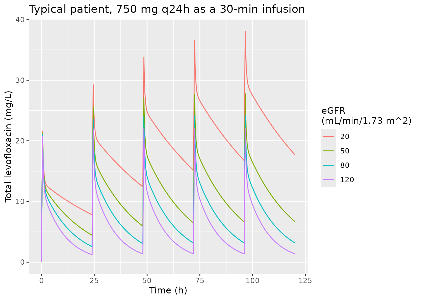

Virtual cohort and stochastic simulation

The cohort below draws eGFR from a log-normal distribution matching the Table 1 mean and SD (52.7 +/- 33.7 mL/min/1.73 m^2), truncated to the 5-150 range, and gives each arm five daily 30-minute infusions. 200 subjects per arm.

rxode2::rxSetSeed(20220527)
n_per_arm <- 200
sdlog <- sqrt(log(1 + (33.7 / 52.7)^2))
meanlog <- log(52.7) - sdlog^2 / 2
draw_egfr <- function(n) {
  x <- rlnorm(4 * n, meanlog, sdlog)
  x <- x[x >= 5 & x <= 150]
  x[seq_len(n)]
}
set.seed(20220527)
cohort <- tibble::tibble(
  id = seq_len(2 * n_per_arm),
  treatment = rep(c("500 mg q24h", "750 mg q24h"), each = n_per_arm),
  dose = rep(c(500, 750), each = n_per_arm),
  CRCL = draw_egfr(2 * n_per_arm)
)
summary(cohort$CRCL)
#>    Min. 1st Qu.  Median    Mean 3rd Qu.    Max. 
#>   9.158  31.112  43.969  51.018  66.100 146.579

ev_vpc <- dplyr::bind_rows(lapply(seq_len(nrow(cohort)), function(i) {
  mk_events(cohort$dose[i], 24, 5, cohort$CRCL[i], id = cohort$id[i],
            t_end = 120, dt = 0.5)
}))

sim_vpc <- rxode2::rxSolve(mod, events = ev_vpc, keep = "CRCL") |>
  as.data.frame() |>
  dplyr::left_join(cohort |> dplyr::select(id, treatment, dose), by = "id")
#> ℹ parameter labels from comments will be replaced by 'label()'

vpc_sum <- sim_vpc |>
  dplyr::group_by(treatment, time) |>
  dplyr::summarise(
    p05 = quantile(Cc, 0.05), p50 = median(Cc), p95 = quantile(Cc, 0.95),
    .groups = "drop"
  )

ggplot(vpc_sum, aes(time, p50)) +
  geom_ribbon(aes(ymin = p05, ymax = p95), alpha = 0.25) +
  geom_line() +
  facet_wrap(~treatment) +
  labs(x = "Time (h)", y = "Total levofloxacin (mg/L)",
       title = "Simulated median and 90% interval, five daily doses",
       caption = paste("Compare with the observed range of Figure 2 of Setiawan 2022",
                       "(observations up to about 35 mg/L, most below 30 mg/L)."))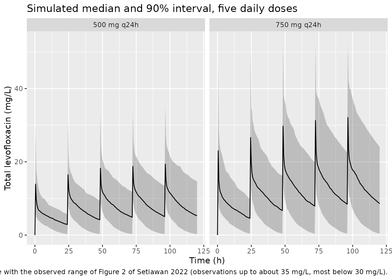

Figure 2 of the paper is a VPC on the study’s own irregular dosing and sampling history, so it cannot be overlaid directly. On the first day the simulated 90% interval one hour after a 750 mg dose (about 8-28 mg/L) lies within the range of the observations, most of which are below 30 mg/L. By day 5, accumulation in patients with low eGFR lifts the 95th percentile to about 50 mg/L, which is later than most of the paper’s samples.

PKNCA validation

The paper reports no NCA table. The NCA is therefore validated against the exact steady-state identity AUC(0-tau) = Dose / CL, applied to the typical-value patient at each eGFR level under a steady-state (ss = 1) regimen. Both sides use the same parameters with no residual error, so the difference is numerical error and a tight bound is correct. The stochastic cohort is then summarised by treatment arm for day 1 and day 5.

ev_ss <- dplyr::bind_rows(lapply(seq_along(egfr_levels), function(i) {
  dplyr::bind_rows(
    data.frame(id = i, time = 0, amt = 750, rate = 1500, evid = 1L, ss = 1L,
               ii = 24, cmt = "central", CRCL = egfr_levels[i]),
    data.frame(id = i, time = c(seq(0, 1, by = 0.05), seq(1.25, 24, by = 0.25)),
               amt = NA_real_, rate = NA_real_, evid = 0L, ss = 0L, ii = 0,
               cmt = "central", CRCL = egfr_levels[i])
  )
}))
sim_ss <- rxode2::rxSolve(rxode2::zeroRe(mod), events = ev_ss, keep = "CRCL",
                          rtol = 1e-10, atol = 1e-12, ssRtol = 1e-10,
                          ssAtol = 1e-12, maxsteps = 1e6) |>
  as.data.frame()
#> ℹ parameter labels from comments will be replaced by 'label()'
#> ℹ omega/sigma items treated as zero: 'etalcl', 'etalvc', 'etalq', 'etalvp'
#> Warning: multi-subject simulation without without 'omega'
stopifnot(all(sim_ss$Cc >= -1e-6 * max(sim_ss$Cc)))

conc_ss <- sim_ss |>
  dplyr::filter(!is.na(Cc)) |>
  dplyr::mutate(Cc = pmax(Cc, 0), treatment = paste0("eGFR ", CRCL))
stopifnot(all(tapply(conc_ss$time == 0, conc_ss$id, any)))
dose_ss <- conc_ss |>
  dplyr::distinct(id, treatment) |>
  dplyr::mutate(time = 0, amt = 750)

nca_ss <- PKNCA::pk.nca(PKNCA::PKNCAdata(
  PKNCA::PKNCAconc(conc_ss, Cc ~ time | treatment + id),
  PKNCA::PKNCAdose(dose_ss, amt ~ time | treatment + id),
  intervals = data.frame(start = 0, end = 24, auclast = TRUE, cmax = TRUE,
                         cmin = TRUE)
))

ss_tab <- as.data.frame(nca_ss) |>
  dplyr::select(treatment, PPTESTCD, PPORRES) |>
  tidyr::pivot_wider(names_from = PPTESTCD, values_from = PPORRES) |>
  dplyr::mutate(
    identity = 750 / (exp(th[["lcl"]]) +
                        th[["e_crcl_cl"]] * as.numeric(sub("eGFR ", "", treatment))),
    err_pct = 100 * (auclast / identity - 1)
  )

knitr::kable(
  ss_tab |>
    dplyr::rename(
      "Typical patient" = treatment, "AUC0-24,ss (mg*h/L)" = auclast,
      "Cmax,ss (mg/L)" = cmax, "Cmin,ss (mg/L)" = cmin,
      "Dose/CL (mg*h/L)" = identity, "Error (%)" = err_pct
    ),
  digits = 3,
  caption = "PKNCA on the typical-value steady-state 750 mg q24h profile against Dose/CL."
)

PKNCA on the typical-value steady-state 750 mg q24h profile against Dose/CL.
Typical patient	AUC0-24,ss (mg*h/L)	Cmax,ss (mg/L)	Cmin,ss (mg/L)	Dose/CL (mg*h/L)	Error (%)
eGFR 120	133.051	22.074	1.373	133.026	0.019
eGFR 20	605.844	40.394	19.079	605.816	0.005
eGFR 50	293.225	27.868	6.725	293.198	0.009
eGFR 80	193.425	24.137	3.178	193.399	0.013


stopifnot(
  nrow(ss_tab) == 4,
  # Linear-up / log-down trapezoids on a 0.05-0.25 h grid; the residual error is
  # the trapezoid rule on the infusion peak, well under 0.1%. A mis-typed slope
  # or intercept moves Dose/CL by tens of percent.
  max(abs(ss_tab$err_pct)) < 0.5
)

conc_vpc <- sim_vpc |>
  dplyr::filter(!is.na(Cc)) |>
  dplyr::mutate(Cc = pmax(Cc, 0))
dose_vpc <- ev_vpc |>
  dplyr::filter(evid == 1) |>
  dplyr::left_join(cohort |> dplyr::select(id, treatment), by = "id") |>
  dplyr::select(id, treatment, time, amt)

nca_vpc <- PKNCA::pk.nca(PKNCA::PKNCAdata(
  PKNCA::PKNCAconc(conc_vpc, Cc ~ time | treatment + id),
  PKNCA::PKNCAdose(dose_vpc, amt ~ time | treatment + id),
  intervals = data.frame(start = c(0, 96), end = c(24, 120), auclast = TRUE,
                         cmax = TRUE, cmin = TRUE)
))

summary(nca_vpc)
#>  start end   treatment   N    auclast        cmax       cmin
#>      0  24 500 mg q24h 200 116 [39.8] 13.4 [52.1]         NC
#>     96 120 500 mg q24h 200 197 [62.6] 19.4 [38.5] 3.71 [209]
#>      0  24 750 mg q24h 200 183 [45.1] 22.0 [54.3]         NC
#>     96 120 750 mg q24h 200 306 [67.7] 31.3 [41.2] 5.46 [245]
#> 
#> Caption: auclast, cmax, cmin: geometric mean and geometric coefficient of variation; N: number of subjects

Replicating the published PTA (Figures 3 and 4)

The paper’s dosing simulations target fAUC0-24/MIC >= 80 with 30% protein binding. At steady state the AUC over a dosing interval is exactly Dose / CL, so for a q24h regimen the steady-state PTA follows in closed form from the model’s own clearance distribution, PTA(MIC) = P(CL <= fu x Dose / (80 x MIC)), with CL log-normal around the eGFR-predicted typical value. That makes the comparison deterministic.

The published points were digitised by the maintainers from panel B (steady state) of Figures 3 and 4; only points strictly inside the 0-1 range are used.

fu <- th[["fu"]]
om_cl <- sqrt(ui$omega["etalcl", "etalcl"])
pta_ss <- function(egfr, dose, mic) {
  tv <- exp(th[["lcl"]]) + th[["e_crcl_cl"]] * egfr
  stats::plnorm(fu * dose / (80 * mic), log(tv), om_cl)
}

pub_ss <- tibble::tribble(
  ~egfr, ~dose, ~mic, ~pta_pub,
  50, 750, 2, 0.73,
  50, 750, 4, 0.18,
  80, 500, 0.5, 0.90,
  80, 500, 1, 0.66,
  80, 500, 2, 0.13,
  80, 750, 1, 0.84,
  80, 750, 2, 0.46,
  80, 750, 4, 0.07,
  80, 1000, 1, 0.90,
  80, 1000, 2, 0.67,
  80, 1000, 4, 0.13,
  120, 500, 0.5, 0.81,
  120, 500, 1, 0.36,
  120, 500, 2, 0.07,
  120, 750, 0.5, 0.91,
  120, 750, 1, 0.68,
  120, 750, 2, 0.15,
  120, 1000, 1, 0.82,
  120, 1000, 2, 0.37,
  120, 1000, 4, 0.08
) |>
  dplyr::mutate(
    pta_model = pta_ss(egfr, dose, mic),
    diff = pta_model - pta_pub
  )

knitr::kable(
  pub_ss |>
    dplyr::rename(
      "eGFR" = egfr, "Dose q24h (mg)" = dose, "MIC (mg/L)" = mic,
      "PTA published (Fig. 3B/4B)" = pta_pub, "PTA model" = pta_model,
      "Difference" = diff
    ),
  digits = 2,
  caption = "Steady-state PTA: closed form from the model against the digitised published curves."
)

Steady-state PTA: closed form from the model against the digitised published curves.
eGFR	Dose q24h (mg)	MIC (mg/L)	PTA published (Fig. 3B/4B)	PTA model	Difference
50	750	2.0	0.73	0.69	-0.04
50	750	4.0	0.18	0.18	0.00
80	500	0.5	0.90	0.95	0.05
80	500	1.0	0.66	0.60	-0.06
80	500	2.0	0.13	0.12	-0.01
80	750	1.0	0.84	0.86	0.02
80	750	2.0	0.46	0.37	-0.09
80	750	4.0	0.07	0.04	-0.03
80	1000	1.0	0.90	0.95	0.05
80	1000	2.0	0.67	0.60	-0.07
80	1000	4.0	0.13	0.12	-0.01
120	500	0.5	0.81	0.82	0.01
120	500	1.0	0.36	0.30	-0.06
120	500	2.0	0.07	0.03	-0.04
120	750	0.5	0.91	0.96	0.05
120	750	1.0	0.68	0.62	-0.06
120	750	2.0	0.15	0.13	-0.02
120	1000	1.0	0.82	0.82	0.00
120	1000	2.0	0.37	0.30	-0.07
120	1000	4.0	0.08	0.03	-0.05


stopifnot(
  nrow(pub_ss) == 20,
  # Deterministic (no simulation). Realised median |diff| 0.046 and maximum
  # 0.094; digitising error is about +/-0.02. The scaling table below shows the
  # bound can go red: scaling clearance by the Table 2 CL mean (1.12) gives a
  # maximum |diff| of 0.18.
  median(abs(pub_ss$diff)) < 0.06,
  max(abs(pub_ss$diff)) < 0.12
)

Which reading of the Table 2 CL row is right (see Assumptions)? Scaling the equation’s typical clearance shows what the paper’s own PTA curves allow:

scale_fit <- tibble::tibble(scale = c(0.90, 1, 1.12)) |>
  dplyr::mutate(
    med = vapply(scale, function(s) {
      median(abs(pta_ss(pub_ss$egfr, pub_ss$dose / s, pub_ss$mic) - pub_ss$pta_pub))
    }, numeric(1)),
    mx = vapply(scale, function(s) {
      max(abs(pta_ss(pub_ss$egfr, pub_ss$dose / s, pub_ss$mic) - pub_ss$pta_pub))
    }, numeric(1)),
    reading = c("Table 2 CL median (0.90) x equation", "Equation as printed (encoded)",
                "Table 2 CL mean (1.12) x equation")
  )
knitr::kable(
  scale_fit |>
    dplyr::select(reading, scale, med, mx) |>
    dplyr::rename("Typical clearance" = reading, "Scale on equation" = scale,
                  "Median |diff|" = med, "Max |diff|" = mx),
  digits = 3,
  caption = "Steady-state PTA fit against the 20 digitised points for three readings of Table 2."
)

Steady-state PTA fit against the 20 digitised points for three readings of Table 2.
Typical clearance	Scale on equation	Median \|diff\|	Max \|diff\|
Table 2 CL median (0.90) x equation	0.90	0.037	0.070
Equation as printed (encoded)	1.00	0.046	0.094
Table 2 CL mean (1.12) x equation	1.12	0.061	0.177

stopifnot(
  # The encoded reading must not be clearly worse than the 0.90 alternative and
  # must beat the 1.12 reading on the worst point.
  scale_fit$mx[2] < scale_fit$mx[3],
  scale_fit$med[2] < scale_fit$med[1] + 0.02
)

ss_curve <- tidyr::expand_grid(
  egfr = c(80, 120), dose = c(500, 750, 1000),
  mic = 2^seq(-3, 3, by = 0.1)
) |>
  dplyr::mutate(pta = pta_ss(egfr, dose, mic))

ggplot(ss_curve, aes(mic, pta, colour = factor(dose))) +
  geom_line() +
  geom_point(data = pub_ss |> dplyr::filter(egfr %in% c(80, 120)),
             aes(y = pta_pub), shape = 1, size = 2) +
  facet_wrap(~ paste("eGFR", egfr)) +
  scale_x_log10() +
  geom_hline(yintercept = 0.9, linetype = "dotted") +
  labs(x = "MIC (mg/L)", y = "PTA (fAUC/MIC >= 80)", colour = "Dose q24h (mg)",
       title = "Replicates Figure 4B of Setiawan 2022 (steady state)",
       caption = "Lines: model closed form. Circles: digitised from the paper.")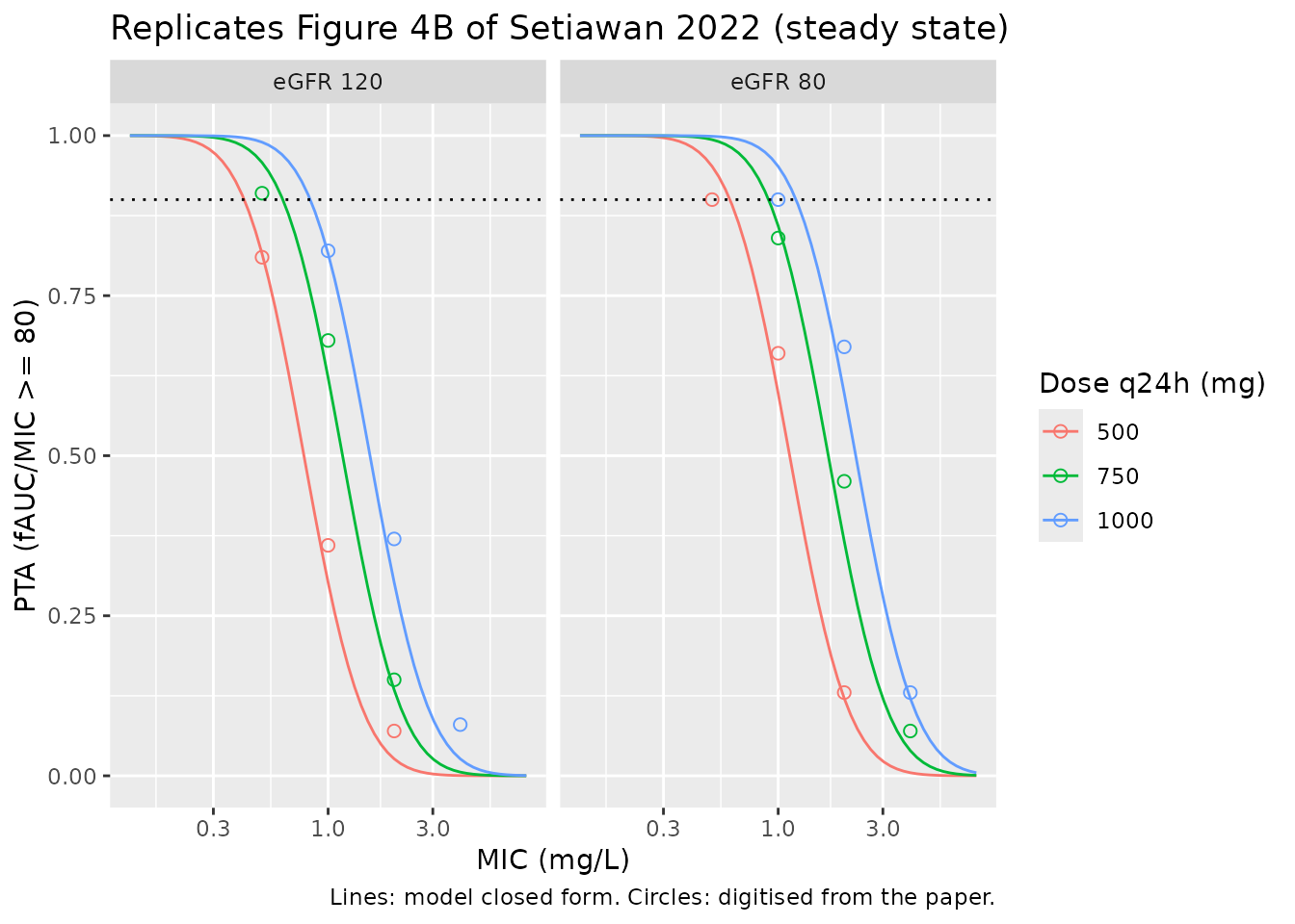

First 24 hours

On day 1 the AUC over 0-24 h also depends on the distribution volumes, so it is simulated: 200 subjects at each of eGFR 80 and 120, given a single 1000 mg 30-minute infusion. Because the model is linear, the AUC for 500 and 750 mg is the 1000 mg AUC scaled by dose, so one cohort per eGFR level serves all three regimens (common random numbers).

rxode2::rxSetSeed(20220528)
ev_d1 <- dplyr::bind_rows(lapply(seq_len(2 * n_per_arm), function(i) {
  mk_events(1000, 24, 1, ifelse(i <= n_per_arm, 80, 120), id = i, t_end = 24,
            dt = 0.25)
}))
sim_d1 <- rxode2::rxSolve(mod, events = ev_d1, keep = "CRCL") |>
  as.data.frame() |>
  dplyr::filter(!is.na(Cc)) |>
  dplyr::mutate(Cc = pmax(Cc, 0), treatment = paste0("eGFR ", CRCL))

nca_d1 <- PKNCA::pk.nca(PKNCA::PKNCAdata(
  PKNCA::PKNCAconc(sim_d1, Cc ~ time | treatment + id),
  PKNCA::PKNCAdose(sim_d1 |> dplyr::distinct(treatment, id) |>
                     dplyr::mutate(time = 0, amt = 1000),
                   amt ~ time | treatment + id),
  intervals = data.frame(start = 0, end = 24, auclast = TRUE)
))
auc_d1 <- as.data.frame(nca_d1) |>
  dplyr::filter(PPTESTCD == "auclast") |>
  dplyr::mutate(egfr = as.numeric(sub("eGFR ", "", treatment))) |>
  dplyr::select(id, egfr, auc1000 = PPORRES)
stopifnot(nrow(auc_d1) == 2 * n_per_arm)

pub_d1 <- tibble::tribble(
  ~egfr, ~dose, ~mic, ~pta_pub, ~source, ~deviation,
  80, 500, 0.5, 0.89, "Fig. 4A", FALSE,
  80, 500, 1, 0.48, "Fig. 4A", TRUE,
  80, 750, 2, 0.08, "Fig. 4A", FALSE,
  80, 1000, 1, 0.88, "Fig. 4A", FALSE,
  80, 1000, 2, 0.49, "Fig. 4A", TRUE,
  120, 500, 0.5, 0.80, "Fig. 4A", FALSE,
  120, 500, 1, 0.16, "Fig. 4A", FALSE,
  120, 750, 0.5, 0.893, "Results text (89.3%)", FALSE,
  120, 1000, 1, 0.71, "Fig. 4A", FALSE,
  120, 1000, 2, 0.16, "Fig. 4A", FALSE
)
pub_d1$pta_model <- vapply(seq_len(nrow(pub_d1)), function(i) {
  a <- auc_d1$auc1000[auc_d1$egfr == pub_d1$egfr[i]] * pub_d1$dose[i] / 1000
  if (length(a) != n_per_arm) stop("no cohort for eGFR ", pub_d1$egfr[i])
  mean(fu * a / pub_d1$mic[i] >= 80)
}, numeric(1))
pub_d1$diff <- pub_d1$pta_model - pub_d1$pta_pub

knitr::kable(
  pub_d1 |>
    dplyr::rename(
      "eGFR" = egfr, "Dose (mg)" = dose, "MIC (mg/L)" = mic,
      "PTA published" = pta_pub, "Source" = source, "PTA model" = pta_model,
      "Difference" = diff, "Known deviation" = deviation
    ),
  digits = 2,
  caption = "First-24-h PTA: simulated cohort (200 per eGFR level) against the published values."
)

First-24-h PTA: simulated cohort (200 per eGFR level) against the published values.
eGFR	Dose (mg)	MIC (mg/L)	PTA published	Source	Known deviation	PTA model	Difference
80	500	0.5	0.89	Fig. 4A	FALSE	0.92	0.03
80	500	1.0	0.48	Fig. 4A	TRUE	0.22	-0.26
80	750	2.0	0.08	Fig. 4A	FALSE	0.04	-0.04
80	1000	1.0	0.88	Fig. 4A	FALSE	0.92	0.04
80	1000	2.0	0.49	Fig. 4A	TRUE	0.22	-0.27
120	500	0.5	0.80	Fig. 4A	FALSE	0.72	-0.09
120	500	1.0	0.16	Fig. 4A	FALSE	0.12	-0.04
120	750	0.5	0.89	Results text (89.3%)	FALSE	0.94	0.04
120	1000	1.0	0.71	Fig. 4A	FALSE	0.72	0.01
120	1000	2.0	0.16	Fig. 4A	FALSE	0.12	-0.04


gated <- pub_d1[!pub_d1$deviation, ]
stopifnot(
  nrow(gated) == 8,
  # Simulated: each model PTA carries a binomial SE of up to 0.035 at n = 200,
  # and the cohort differs across rxode2 builds and thread counts, so gate on
  # the centre of the differences with headroom over that noise.
  abs(median(gated$diff)) < 0.08,
  max(abs(gated$diff)) < 0.20,
  # The two known deviations stay visibly low; if they ever reproduce, revisit
  # the explanation below.
  all(pub_d1$diff[pub_d1$deviation] < 0)
)

Known deviation. At eGFR 80 the model’s first-day PTA sits well below the published curve in the middle of its fall (about 0.2-0.3 lower at MIC 1 mg/L for 500 mg and MIC 2 mg/L for 1000 mg), while the end points of the curve, the eGFR 120 panel and every steady-state point agree. Steady-state PTA depends on clearance alone, whereas day-1 AUC also depends on how fast a subject reaches its terminal phase. With independent etas, the low-clearance subjects who pass the target are often ones with large volumes and long half-lives, and these accumulate least on day 1. NPAG estimates the joint density of all four parameters, including covariances the paper does not report. A positive CL-V correlation would remove that penalty. As a sensitivity check, the chunk below removes the volume and Q variability altogether and re-simulates the eGFR 80 cohort. That raises the two deviating PTAs toward the published values, which supports the mechanism, but does not close the gap. The rest cannot be reproduced from the published summary statistics, and the parameters have not been tuned to it.

mod_cl_only <- mod |>
  rxode2::ini(etalvc ~ 1e-6, etalq ~ 1e-6, etalvp ~ 1e-6)
#> ℹ parameter labels from comments will be replaced by 'label()'
#> ℹ change initial estimate of `etalvc` to `1e-06`
#> ℹ change initial estimate of `etalq` to `1e-06`
#> ℹ change initial estimate of `etalvp` to `1e-06`
rxode2::rxSetSeed(20220529)
sim_s <- rxode2::rxSolve(mod_cl_only,
                         events = ev_d1[ev_d1$id <= n_per_arm, ],
                         keep = "CRCL") |>
  as.data.frame() |>
  dplyr::filter(!is.na(Cc)) |>
  dplyr::group_by(id) |>
  dplyr::summarise(auc1000 = sum(diff(time) * (head(Cc, -1) + tail(Cc, -1)) / 2))
sens <- pub_d1 |>
  dplyr::filter(deviation) |>
  dplyr::mutate(pta_cl_only = vapply(seq_len(dplyr::n()), function(i) {
    mean(fu * sim_s$auc1000 * dose[i] / 1000 / mic[i] >= 80)
  }, numeric(1)))
knitr::kable(
  sens |>
    dplyr::select(egfr, dose, mic, pta_pub, pta_model, pta_cl_only) |>
    dplyr::rename("eGFR" = egfr, "Dose (mg)" = dose, "MIC (mg/L)" = mic,
                  "PTA published" = pta_pub, "PTA model" = pta_model,
                  "PTA, IIV on CL only" = pta_cl_only),
  digits = 2,
  caption = "Day-1 PTA at the two deviating points with and without volume/Q IIV."
)

Day-1 PTA at the two deviating points with and without volume/Q IIV.
eGFR	Dose (mg)	MIC (mg/L)	PTA published	PTA model	PTA, IIV on CL only
80	500	1	0.48	0.22	0.38
80	1000	2	0.49	0.22	0.38

Assumptions and deviations

Typical clearance is the printed equation, not the Table 2 CL row. The Results state that “the CL of levofloxacin was best described as CL = (0.044 x eGFR CKD-EPI) + 0.358”, and that is encoded verbatim. Table 2 separately lists CL with mean 1.12 L/h, median 0.90 L/h and CV 52%, and the Abstract and Discussion quote 1.12 L/h as “the population estimate for clearance”. The two cannot both be the clearance of a typical patient: the equation reaches 1.12 L/h only at eGFR 17 mL/min/1.73 m^2, against a cohort mean of 52.7. The most likely explanation is that the Pmetrics model multiplied a random scaling factor (median 0.90, close to 1) by the eGFR relationship, which the paper does not state. The paper’s own steady-state PTA curves settle what matters in practice (table in the PTA section). With the equation as the typical clearance and a 52% CV, the closed-form PTA reproduces the 20 digitised points with a median absolute difference of about 0.05. Scaling by the median 0.90 fits about as well, within digitising error. Scaling by the mean 1.12 fits worse, with a worst point 0.18 off. The printed equation is therefore kept unscaled, and the CV% is kept as the IIV on clearance.
Volumes and Q use the Table 2 MEANS, the values quoted in the Abstract and the convention of the same group’s ampicillin-sulbactam model (Setiawan_2023_sulbactam). The medians differ by at most 7% (Q 33.2 vs 30.9 L/h).
IIV is a log-normal approximation to the non-parametric NPAG density, omega^2 = log(CV^2 + 1), with independent etas because no covariances are reported. Whatever shape the joint density has, including any multimodality, cannot be recovered from the published tables.
Residual error is fixed to zero. The selected lambda/gamma error model and the assay-error polynomial are not reported in the paper or its supplement. Simulated concentrations are therefore error-free individual predictions.
Covariate scope. Only eGFR is used; it is the CKD-EPI creatinine equation in mL/min/1.73 m^2 and is passed as CRCL. Sex, serum creatinine, ICU admission and mechanical ventilation were screened and not retained, and are recorded under covariatesDataExcluded. The linear relationship has no floor, so the model should not be used outside the range observed or for patients on renal replacement therapy.
Virtual cohort. The VPC cohort draws eGFR log-normally to match the Table 1 mean and SD, truncated to 5-150 mL/min/1.73 m^2. The paper does not report the eGFR range.
Steady state in the paper. The authors evaluated “steady state” on the fifth treatment day. At eGFR 20 the typical terminal half-life exceeds a day (table above), so day 5 is not yet at steady state there. The closed-form comparison above therefore uses only q24h regimens at eGFR 50, 80 and 120.
Digitised values. The published PTA points were read by the maintainers from Figures 3B, 4A and 4B to about +/-0.02. One first-day value (89.3%, 750 mg q24h, eGFR 120, MIC 0.5 mg/L) is printed in the Results.

Errata

No erratum or correction to Setiawan 2022 was found in a Europe PMC search (checked 2026-10-01). Two internal inconsistencies of the paper are noted:

The Table 2 CL row (mean 1.12 L/h) disagrees with the printed CL equation; see the first item above.
Table 1 reports albumin as “2.80 +/- 0.50 g/l”, which is consistent with g/dL. Albumin is not a model covariate.