Meloxicam nanocapsules in dogs (Teixeira 2026)
Source:vignettes/articles/Teixeira_2026_meloxicam_dog.Rmd
Teixeira_2026_meloxicam_dog.RmdModel and source
- Citation: Teixeira FEG, Lock GA, Giacomeli R, Pacheco CO, Maciel TR, Funghetto-Ribeiro AP, Lugoch G, Beckmann DV, de Oliveira MT, Haas SE. Evaluating orally administered meloxicam-loaded polymeric nanocapsules in female dogs: a population pharmacokinetic modeling study. Pharmaceuticals (Basel). 2026;19(3):412. doi:10.3390/ph19030412.
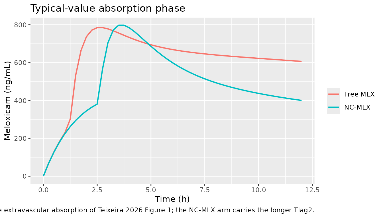
- Description: Preclinical (dog). Two-compartment population PK model for meloxicam in 18 female mixed-breed dogs undergoing elective ovariohysterectomy, after a single 0.2 mg/kg oral dose of either a free meloxicam solution or meloxicam-loaded poly(epsilon-caprolactone) polymeric nanocapsules (Teixeira 2026). Absorption is a double extravascular process: a fraction F1 of the dose enters depot and is absorbed with a slow first-order rate ka1, while the remaining 1 - F1 enters depot2 and is absorbed with a much faster first-order rate ka2 after a lag time Tlag2 - the structure the authors used to describe the secondary plasma peak seen in several animals. The nanocapsule formulation is a covariate on Tlag2 (2.1-fold longer) and on the apparent peripheral volume V2 (3.0-fold larger); clearance, central volume and both absorption rate constants are unaffected.
- Article: https://doi.org/10.3390/ph19030412
- Supplementary material (Tables S1-S3, Figures S1-S5): https://www.mdpi.com/1424-8247/19/3/412/s1
Population
Eighteen healthy female mixed-breed dogs (9 per arm) aged 9-48 months and weighing 10.5-16.6 kg were recruited from the UNIPAMPA Veterinary Hospital (Uruguaiana, Rio Grande do Sul, Brazil) and hospitalised 24 h before elective ovariohysterectomy. Each dog received a single 0.2 mg/kg oral dose of meloxicam 4 h before surgery, as either the free-drug solution (meloxicam in 60% v/v PEG-400, 0.5 mg/mL, 5.2 +/- 0.4 mL administered) or the poly(epsilon-caprolactone) nanocapsule suspension NC-MLX (1 mg/mL, 2.8 +/- 0.3 mL administered). Plasma was sampled at 0.5, 1, 2, 4, 6, 8, 12, 24, 36, 48 and 60 h post-dose and assayed by HPLC-PDA against a piroxicam internal standard, giving 196 observations, all above the quantification limit (Teixeira 2026 Section 4.4-4.6).
Baseline characteristics differed only slightly between arms (supplementary Table S1): body weight 14.2 +/- 1.6 kg (free MLX) vs 12.9 +/- 1.8 kg (NC-MLX) and age 26.1 +/- 18.3 vs 19.5 +/- 14.4 months. Age and weight were both screened as covariates (Table S2) but only formulation was retained in the final model.
The same information is available programmatically via the model’s
population metadata
(readModelDb("Teixeira_2026_meloxicam_dog")()$population).
Source trace
The per-parameter origin is recorded as an in-file comment next to
each ini() entry in
inst/modeldb/specificDrugs/Teixeira_2026_meloxicam_dog.R.
The table below collects them in one place for review.
| Equation / parameter | Value | Source location |
|---|---|---|
| Model structure (2 compartments, double extravascular absorption, F1 / 1-F1 dose split, Tlag2 on the second route) | n/a | Figure 1 (final model structure diagram) and Section 2.3 |
lka (ka1) |
0.086 1/h | Table 2, Ka1_pop (RSE 20.1%) |
lka2 (ka2) |
1.82 1/h | Table 2, Ka2_pop (RSE 51.3%) |
logitfdepot (F1) |
0.85 | Table 2, F1_pop (RSE 5.87%) |
ltlag2 (Tlag2, free MLX) |
1.22 h | Table 2, Tlag2_pop (RSE 16.3%); restated in Section
2.3 |
lcl (CL/F) |
0.1 mL/min/kg = 0.006 L/h/kg | Table 2, CL_pop (RSE 8.56%); unit confirmed against
Table 1 CL/F
|
lvc (V1/F) |
0.049 L/kg | Table 2, V1_pop (RSE 56.0%) |
lq (Q) |
0.24 L/h | Table 2, Q_pop (RSE 24.1%) |
lvp (V2/F, free MLX) |
0.134 L/kg | Table 2, V2_pop (RSE 27.8%) |
e_form_nanocapsule_tlag2 |
0.74 | Table 2, beta_Tlag2_NC-MLX (RSE 28.7%) |
e_form_nanocapsule_vp |
1.11 | Table 2, beta_V2_NC-MLX (RSE 31.4%) |
etalka |
omega 0.38 -> var 0.1444 | Table 2, omega Ka1 (RSE 21.1%) |
etalka2 |
omega 1.28 -> var 1.6384 | Table 2, omega Ka2 (RSE 35.3%) |
etalogitfdepot |
omega 0.67 -> var 0.4489 | Table 2, omega F1 (RSE 53.8%) |
etaltlag2 |
omega 0.38 -> var 0.1444 | Table 2, omega Tlag2 (RSE 20.7%) |
etalcl |
omega 0.32 -> var 0.1024 | Table 2, omega CL (RSE 19.4%) |
etalvc |
omega 1.44 -> var 2.0736 | Table 2, omega V1 (RSE 29.8%) |
etalvp |
omega 0.65 -> var 0.4225 | Table 2, omega V2 (RSE 20.3%) |
| No IIV on Q | n/a | Section 2.3: “Interindividual variability was maintained for all PK parameters except Q” |
propSd |
0.19 | Table 2, “Proportional model” (RSE 6.83%); Section 2.3 |
Exponential IIV, P_i = P_pop * exp(eta_i)
|
n/a | Section 4.6.2, Equation (1) |
| Reference NCA (Table 1 transcription below) | see table | Table 1 |
| Demographics | see Population | Supplementary Table S1 |
| Covariate screen (age, weight, formulation) | n/a | Section 4.6.2; supplementary Table S2 footnotes a/b/c |
Virtual cohort
Original observed data are not publicly available. The cohort below reproduces the arm-specific weight distributions of supplementary Table S1, truncated to the published overall weight range of 10.5-16.6 kg, with 100 dogs per arm.
Because Table 2 reports CL_pop, V1_pop and
V2_pop per kilogram of body weight while Q_pop
is reported in absolute L/h, the packaged model multiplies the per-kg
clearance and volumes by WT. The dose is therefore entered
in milligrams, as 0.2 * WT.
set.seed(20260830)

n_per_arm <- 100L
obs_times <- seq(0, 60, by = 0.5)
# The paper's actual sampling schedule (Section 4.4). NCA is run on these
# nominal times only, so the simulated and published NCA are computed from
# concentration-time profiles of the same resolution.
nominal_times <- c(0, 0.5, 1, 2, 4, 6, 8, 12, 24, 36, 48, 60)

make_arm <- function(n, label, nano, wt_mean, wt_sd, id_offset) {
  wt <- pmin(pmax(stats::rnorm(n, wt_mean, wt_sd), 10.5), 16.6)
  subj <- tibble::tibble(
    id                   = id_offset + seq_len(n),
    treatment            = label,
    WT                   = wt,
    FORM_MLX_NANOCAPSULE = nano,
    dose_mg              = 0.2 * wt
  )
  # Both depots receive the same total dose amount; f(depot) = F1 and
  # f(depot2) = 1 - F1 partition it (Teixeira 2026 Figure 1).
  dose_rows <- dplyr::bind_rows(
    subj |> dplyr::mutate(time = 0, amt = dose_mg, evid = 1L, cmt = "depot"),
    subj |> dplyr::mutate(time = 0, amt = dose_mg, evid = 1L, cmt = "depot2")
  )
  obs_rows <- subj |>
    tidyr::crossing(time = obs_times) |>
    dplyr::mutate(amt = NA_real_, evid = 0L, cmt = "central")
  dplyr::bind_rows(dose_rows, obs_rows) |>
    dplyr::arrange(id, time, dplyr::desc(evid)) |>
    dplyr::select(id, time, amt, evid, cmt, treatment, WT, FORM_MLX_NANOCAPSULE)
}

events <- dplyr::bind_rows(
  make_arm(n_per_arm, "Free MLX", 0, 14.2, 1.6, id_offset = 0L),
  make_arm(n_per_arm, "NC-MLX",   1, 12.9, 1.8, id_offset = n_per_arm)
)

stopifnot(
  !anyDuplicated(events[events$evid == 0L, c("id", "time")]),
  nrow(dplyr::distinct(events, id)) == 2L * n_per_arm
)
Simulation
mod <- readModelDb("Teixeira_2026_meloxicam_dog")

sim <- rxode2::rxSolve(
  mod, events = events,
  keep        = c("treatment", "WT", "FORM_MLX_NANOCAPSULE"),
  addDosing   = FALSE,
  useLinCmt   = FALSE
) |>
  as.data.frame()
#> ℹ parameter labels from comments will be replaced by 'label()'

stopifnot(nrow(sim) > 0, !all(is.na(sim$Cc)))
A second, deterministic simulation with the random effects zeroed
reproduces the typical-value profile of each arm and is used for the
structural identity checks below. It runs on a long horizon so that
AUC(0-inf) is essentially complete.
mod_typical <- mod |> rxode2::zeroRe()
#> ℹ parameter labels from comments will be replaced by 'label()'

typ_subj <- tibble::tibble(
  id                   = 1:2,
  treatment            = c("Free MLX", "NC-MLX"),
  WT                   = c(14.2, 12.9),
  FORM_MLX_NANOCAPSULE = c(0, 1),
  dose_mg              = 0.2 * c(14.2, 12.9)
)

typ_events <- dplyr::bind_rows(
  typ_subj |> dplyr::mutate(time = 0, amt = dose_mg, evid = 1L, cmt = "depot"),
  typ_subj |> dplyr::mutate(time = 0, amt = dose_mg, evid = 1L, cmt = "depot2"),
  typ_subj |>
    tidyr::crossing(time = seq(0, 600, by = 0.25)) |>
    dplyr::mutate(amt = NA_real_, evid = 0L, cmt = "central")
) |>
  dplyr::arrange(id, time, dplyr::desc(evid)) |>
  dplyr::select(id, time, amt, evid, cmt, treatment, WT, FORM_MLX_NANOCAPSULE)

sim_typical <- rxode2::rxSolve(
  mod_typical, events = typ_events,
  keep      = c("treatment", "WT", "FORM_MLX_NANOCAPSULE"),
  addDosing = FALSE,
  useLinCmt = FALSE
) |>
  as.data.frame()
#> ℹ omega/sigma items treated as zero: 'etalka', 'etalka2', 'etalogitfdepot', 'etaltlag2', 'etalcl', 'etalvc', 'etalvp'
#> Warning: multi-subject simulation without without 'omega'
Structural checks
Covariate effects on Tlag2 and V2
The formulation coefficients enter additively on the log scale, so
the packaged model must reproduce the two values the paper states in
prose (Section 2.3): Tlag2 1.22 h (free MLX) vs 2.55 h
(NC-MLX), and V2 0.134 L/kg (free MLX) vs 0.406 L/kg
(NC-MLX).
cov_chk <- sim_typical |>
  dplyr::group_by(treatment) |>
  dplyr::summarise(
    tlag2      = unique(round(tlag2, 10)),
    vp_per_kg  = unique(round(vp / WT, 10)),
    .groups    = "drop"
  ) |>
  dplyr::mutate(
    published_tlag2     = c(1.22, 1.22 * exp(0.74)),
    published_vp_per_kg = c(0.134, 0.134 * exp(1.11))
  )

knitr::kable(
  cov_chk |>
    dplyr::mutate(dplyr::across(where(is.numeric), ~ signif(.x, 5))) |>
    dplyr::rename(
      "Arm"                     = treatment,
      "Tlag2 model (h)"         = tlag2,
      "V2 model (L/kg)"         = vp_per_kg,
      "Tlag2 Table 2 (h)"       = published_tlag2,
      "V2 Table 2 (L/kg)"       = published_vp_per_kg
    ),
  caption = "Formulation covariate effects reproduced from Teixeira 2026 Table 2."
)| Arm | Tlag2 model (h) | V2 model (L/kg) | Tlag2 Table 2 (h) | V2 Table 2 (L/kg) |
|---|---|---|---|---|
| Free MLX | 1.220 | 0.1340 | 1.220 | 0.1340 |
| NC-MLX | 2.557 | 0.4066 | 2.557 | 0.4066 |
# Deterministic identities: both sides use the same fixed effects, so the
# tolerance is pure floating-point noise.
stopifnot(
  all(abs(cov_chk$tlag2 / cov_chk$published_tlag2 - 1) < 1e-8),
  all(abs(cov_chk$vp_per_kg / cov_chk$published_vp_per_kg - 1) < 1e-8),
  # The paper's stated NC-MLX values, to the precision it prints them.
  abs(cov_chk$tlag2[cov_chk$treatment == "NC-MLX"] - 2.55) < 0.01,
  abs(cov_chk$vp_per_kg[cov_chk$treatment == "NC-MLX"] - 0.406) < 0.001
)
Mass balance: AUC(0-inf) = Dose / CL
The two absorption routes carry F1 and
1 - F1 of the dose, so all of the administered amount
reaches the central compartment and AUC(0-inf) must equal
Dose / CL exactly. With CL = 0.006 L/h/kg and
a 0.2 mg/kg dose this is
0.2 / 0.006 = 33.3 ug*h/mL in both arms,
because formulation is not a covariate on clearance. This is the
strongest available check that the dose split, the lag time and the
peripheral compartment are all wired correctly.
typ_conc <- sim_typical |>
  dplyr::filter(!is.na(Cc)) |>
  dplyr::select(id, time, Cc, treatment)

typ_dose <- typ_events |>
  dplyr::filter(evid == 1L, cmt == "depot") |>
  dplyr::select(id, time, amt, treatment)

typ_nca <- PKNCA::pk.nca(PKNCA::PKNCAdata(
  PKNCA::PKNCAconc(typ_conc, Cc ~ time | treatment + id),
  PKNCA::PKNCAdose(typ_dose, amt ~ time | treatment + id),
  intervals = data.frame(start = 0, end = Inf, aucinf.obs = TRUE)
))

auc_chk <- as.data.frame(typ_nca) |>
  dplyr::filter(PPTESTCD == "aucinf.obs") |>
  dplyr::select(treatment, id, auc_pknca = PPORRES) |>
  dplyr::left_join(
    sim_typical |>
      dplyr::group_by(treatment, id) |>
      dplyr::summarise(cl = unique(cl), WT = unique(WT), .groups = "drop"),
    by = c("treatment", "id")
  ) |>
  dplyr::mutate(
    auc_analytic = (0.2 * WT) / cl,
    pct_diff     = 100 * (auc_pknca - auc_analytic) / auc_analytic
  )

knitr::kable(
  auc_chk |>
    dplyr::select(treatment, auc_pknca, auc_analytic, pct_diff) |>
    dplyr::mutate(dplyr::across(where(is.numeric), ~ signif(.x, 5))) |>
    dplyr::rename(
      "Arm"                        = treatment,
      "AUC0-inf, PKNCA (ug*h/mL)"  = auc_pknca,
      "Dose / CL (ug*h/mL)"        = auc_analytic,
      "Difference (%)"             = pct_diff
    ),
  caption = "AUC(0-inf) from the typical-value solve vs the closed-form Dose / CL."
)| Arm | AUC0-inf, PKNCA (ug*h/mL) | Dose / CL (ug*h/mL) | Difference (%) |
|---|---|---|---|
| Free MLX | 33.330 | 33.333 | -0.0105320 |
| NC-MLX | 33.331 | 33.333 | -0.0060568 |
stopifnot(
  # Same drawn parameters on both sides -- the residual is trapezoidal and
  # lambda-z extrapolation error only, so a tight all() bound is correct here.
  all(abs(auc_chk$pct_diff) < 1),
  # Clearance carries no formulation covariate, so the two arms must agree.
  abs(diff(auc_chk$auc_analytic)) < 1e-8
)
Replicate published figures
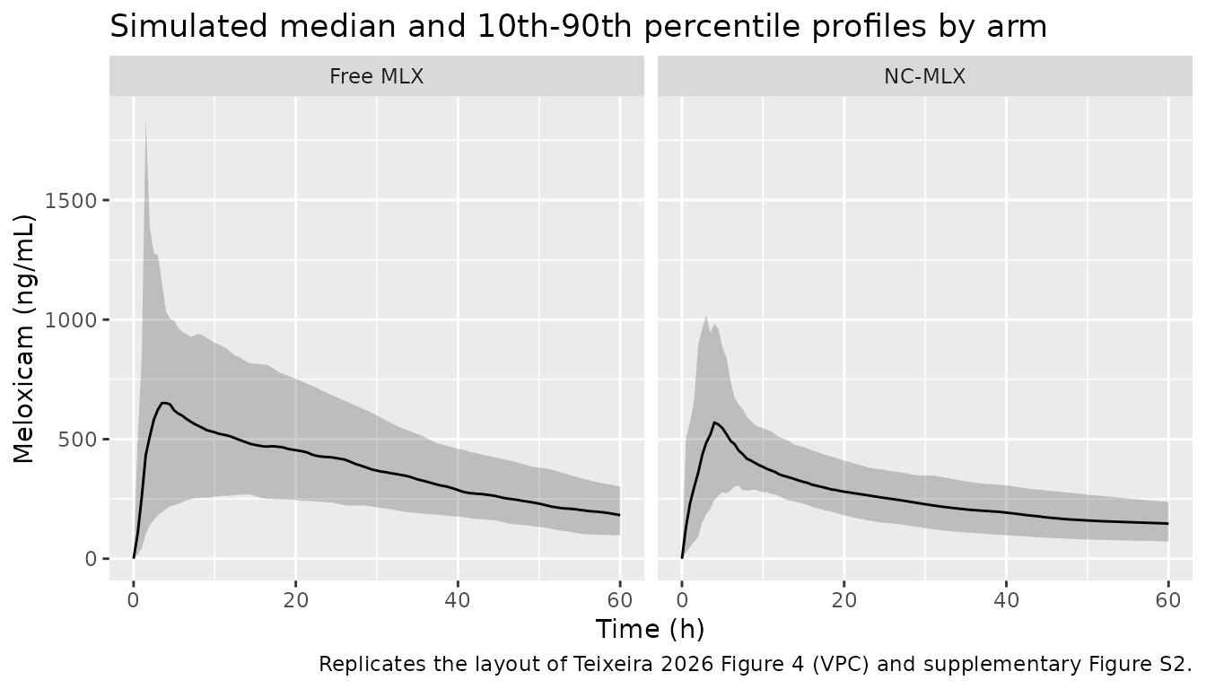
# Replicates supplementary Figure S2 / Figure 4 of Teixeira 2026: observed and
# predicted plasma meloxicam by formulation arm, plotted as ng/mL to match the
# published axis.
sim |>
  dplyr::filter(!is.na(Cc)) |>
  dplyr::group_by(treatment, time) |>
  dplyr::summarise(
    Q10 = stats::quantile(Cc, 0.10) * 1000,
    Q50 = stats::quantile(Cc, 0.50) * 1000,
    Q90 = stats::quantile(Cc, 0.90) * 1000,
    .groups = "drop"
  ) |>
  ggplot2::ggplot(ggplot2::aes(time, Q50)) +
  ggplot2::geom_ribbon(ggplot2::aes(ymin = Q10, ymax = Q90), alpha = 0.25) +
  ggplot2::geom_line() +
  ggplot2::facet_wrap(~treatment) +
  ggplot2::labs(
    x = "Time (h)", y = "Meloxicam (ng/mL)",
    title = "Simulated median and 10th-90th percentile profiles by arm",
    caption = "Replicates the layout of Teixeira 2026 Figure 4 (VPC) and supplementary Figure S2."
  )
# Illustrates the double-absorption structure of Figure 1: the typical-value
# profile of each arm over the first 12 h, where the lagged fast route (ka2)
# produces the secondary absorption wave the authors modelled.
sim_typical |>
  dplyr::filter(!is.na(Cc), time <= 12) |>
  ggplot2::ggplot(ggplot2::aes(time, Cc * 1000, colour = treatment)) +
  ggplot2::geom_line(linewidth = 0.8) +
  ggplot2::labs(
    x = "Time (h)", y = "Meloxicam (ng/mL)", colour = NULL,
    title = "Typical-value absorption phase",
    caption = "Double extravascular absorption of Teixeira 2026 Figure 1; the NC-MLX arm carries the longer Tlag2."
  )
PKNCA validation
NCA is run on the paper’s nominal sampling schedule (0.5-60 h) so that the simulated and published non-compartmental parameters are derived from concentration-time profiles of the same resolution and over the same window.
Typical-value NCA (primary comparison)
Teixeira 2026 Table 1 reports the mean of nine dogs per arm. The corresponding model quantity is the typical-value profile, so this is the primary comparison. The stochastic cohort follows below, and differs for a reason that is a property of the published parameter set rather than of the transcription - see the Errata.
typ_nca_conc <- sim_typical |>
  dplyr::filter(!is.na(Cc), time %in% nominal_times) |>
  dplyr::select(id, time, Cc, treatment)

typ_nca_dose <- typ_events |>
  dplyr::filter(evid == 1L, cmt == "depot") |>
  dplyr::select(id, time, amt, treatment)

nca_intervals <- data.frame(
  start = 0, end = 60,
  cmax = TRUE, tmax = TRUE, auclast = TRUE, half.life = TRUE
)

typ_wide <- as.data.frame(PKNCA::pk.nca(PKNCA::PKNCAdata(
  PKNCA::PKNCAconc(typ_nca_conc, Cc ~ time | treatment + id),
  PKNCA::PKNCAdose(typ_nca_dose, amt ~ time | treatment + id),
  intervals = nca_intervals
))) |>
  dplyr::filter(PPTESTCD %in% c("cmax", "tmax", "auclast", "half.life")) |>
  tidyr::pivot_wider(
    id_cols = treatment, names_from = PPTESTCD, values_from = PPORRES
  )

published <- tibble::tribble(
  ~treatment,  ~cmax, ~tmax, ~auclast, ~half.life,
  "Free MLX",  1.33,  1.83,  23.59,    15.22,
  "NC-MLX",    0.79,  4.37,  19.87,    36.99
)

knitr::kable(
  nlmixr2lib::ncaComparisonTable(
    simulated     = typ_wide,
    reference     = published,
    by            = "treatment",
    units         = c(cmax = "ug/mL", auclast = "ug*h/mL",
                      tmax = "h", half.life = "h"),
    tolerance_pct = 20
  ),
  caption = "Typical-value simulation vs Teixeira 2026 Table 1. * differs from the reference by more than 20%.",
  align   = c("l", "l", "r", "r", "r")
)| NCA parameter | treatment | Reference | Simulated | % diff |
|---|---|---|---|---|
| Cmax (ug/mL) | Free MLX | 1.33 | 0.737 | -44.6%* |
| Cmax (ug/mL) | NC-MLX | 0.79 | 0.784 | -0.8% |
| Tmax (h) | Free MLX | 1.83 | 2 | +9.3% |
| Tmax (h) | NC-MLX | 4.37 | 4 | -8.5% |
| AUClast (ug*h/mL) | Free MLX | 23.6 | 25.7 | +9.1% |
| AUClast (ug*h/mL) | NC-MLX | 19.9 | 17.6 | -11.7% |
| t½ (h) | Free MLX | 15.2 | 27 | +77.3%* |
| t½ (h) | NC-MLX | 37 | 53.5 | +44.7%* |
typ_free <- typ_wide[typ_wide$treatment == "Free MLX", ]
typ_nc   <- typ_wide[typ_wide$treatment == "NC-MLX", ]
pub_free <- published[published$treatment == "Free MLX", ]
pub_nc   <- published[published$treatment == "NC-MLX", ]

stopifnot(
  # Tmax: the model reproduces both published means to within one nominal
  # sampling interval, and reproduces the direction of the formulation effect.
  abs(typ_free$tmax - pub_free$tmax) < 1,
  abs(typ_nc$tmax   - pub_nc$tmax)   < 1,
  typ_nc$tmax > typ_free$tmax,
  # AUC(0-60 h): within 20% in both arms.
  abs(typ_free$auclast / pub_free$auclast - 1) < 0.2,
  abs(typ_nc$auclast   / pub_nc$auclast   - 1) < 0.2,
  # Cmax: asserted only for NC-MLX. The free-MLX Cmax is under-predicted by
  # the published model itself (see Errata), so a tight bound there would be
  # testing the paper, not the transcription.
  abs(typ_nc$cmax / pub_nc$cmax - 1) < 0.2,
  # Terminal half-life is over-predicted in both arms by a similar factor, so
  # the between-arm ratio - the paper's headline 2.4-fold prolongation - is
  # the quantity that survives.
  abs((typ_nc$half.life / typ_free$half.life) / (pub_nc$half.life / pub_free$half.life) - 1) < 0.3
)
Stochastic cohort NCA
sim_nca <- sim |>
  dplyr::filter(!is.na(Cc)) |>
  dplyr::filter(time %in% nominal_times) |>
  dplyr::select(id, time, Cc, treatment)

# Guarantee a time = 0 record per subject; pre-dose Cc = 0 for an oral dose.
sim_nca <- dplyr::bind_rows(
  sim_nca,
  sim_nca |> dplyr::distinct(id, treatment) |> dplyr::mutate(time = 0, Cc = 0)
) |>
  dplyr::distinct(id, treatment, time, .keep_all = TRUE) |>
  dplyr::arrange(id, treatment, time)

dose_df <- events |>
  dplyr::filter(evid == 1L, cmt == "depot") |>
  dplyr::select(id, time, amt, treatment)

nca_res <- PKNCA::pk.nca(PKNCA::PKNCAdata(
  PKNCA::PKNCAconc(sim_nca, Cc ~ time | treatment + id),
  PKNCA::PKNCAdose(dose_df, amt ~ time | treatment + id),
  intervals = nca_intervals
))
#> Warning: Too few points for half-life calculation (min.hl.points=3 with only 2 points)
#> Too few points for half-life calculation (min.hl.points=3 with only 2 points)
#> Too few points for half-life calculation (min.hl.points=3 with only 2 points)
#> Warning: Too few points for half-life calculation (min.hl.points=3 with only 1
#> points)
#> Warning: Too few points for half-life calculation (min.hl.points=3 with only 2 points)
#> Too few points for half-life calculation (min.hl.points=3 with only 2 points)
#> Too few points for half-life calculation (min.hl.points=3 with only 2 points)

nca_wide <- as.data.frame(nca_res) |>
  dplyr::filter(PPTESTCD %in% c("cmax", "tmax", "auclast", "half.life")) |>
  tidyr::pivot_wider(
    id_cols     = c(treatment, id),
    names_from  = PPTESTCD,
    values_from = PPORRES
  )
Teixeira 2026 Table 1 reports arithmetic means, so the cohort is
aggregated the same way before comparison
(ncaComparisonTable() would otherwise take medians, which
are not the published statistic).
simulated_mean <- nca_wide |>
  dplyr::group_by(treatment) |>
  dplyr::summarise(
    dplyr::across(c(cmax, tmax, auclast, half.life), ~ mean(.x, na.rm = TRUE)),
    .groups = "drop"
  )

knitr::kable(
  nlmixr2lib::ncaComparisonTable(
    simulated     = simulated_mean,
    reference     = published,
    by            = "treatment",
    units         = c(cmax = "ug/mL", auclast = "ug*h/mL",
                      tmax = "h", half.life = "h"),
    tolerance_pct = 20
  ),
  caption = "Stochastic cohort (arm mean, n = 100 per arm) vs Teixeira 2026 Table 1. * differs from the reference by more than 20%.",
  align   = c("l", "l", "r", "r", "r")
)| NCA parameter | treatment | Reference | Simulated | % diff |
|---|---|---|---|---|
| Cmax (ug/mL) | Free MLX | 1.33 | 0.944 | -29.0%* |
| Cmax (ug/mL) | NC-MLX | 0.79 | 0.724 | -8.4% |
| Tmax (h) | Free MLX | 1.83 | 8.58 | +368.9%* |
| Tmax (h) | NC-MLX | 4.37 | 5.86 | +34.1%* |
| AUClast (ug*h/mL) | Free MLX | 23.6 | 23.2 | -1.7% |
| AUClast (ug*h/mL) | NC-MLX | 19.9 | 16 | -19.6% |
| t½ (h) | Free MLX | 15.2 | 37.5 | +146.5%* |
| t½ (h) | NC-MLX | 37 | 54.4 | +47.0%* |
Assertions on the paper’s actual claims
Each contrast is asserted at the level where the corresponding parameter lives. The formulation effect is a fixed effect, so its direction and magnitude are checked on the deterministic typical-value profiles. The stochastic cohort is summarised by medians - never by extremes, which are not reproducible across rxode2 releases - and only the direction of each contrast is asserted there.
med <- nca_wide |>
  dplyr::group_by(treatment) |>
  dplyr::summarise(
    dplyr::across(c(cmax, tmax, auclast, half.life), ~ stats::median(.x, na.rm = TRUE)),
    .groups = "drop"
  )

nc   <- med[med$treatment == "NC-MLX", ]
free <- med[med$treatment == "Free MLX", ]

ratio_fmt <- function(x) ifelse(is.na(x), "n/a", sprintf("%.2f-fold", x))

claims <- tibble::tibble(
  Claim = c(
    "Tmax longer with NC-MLX (Table 1: 1.83 -> 4.37 h, p < 0.05)",
    "Terminal half-life longer with NC-MLX (Table 1: 15.22 -> 36.99 h, p < 0.05)",
    "Cmax lower with NC-MLX (Table 1: 1.33 -> 0.79 ug/mL, NOT significant; not reproduced - see Errata)",
    "AUC(0-inf) unchanged by formulation (CL has no formulation covariate)"
  ),
  Published = ratio_fmt(c(
    pub_nc$tmax / pub_free$tmax,
    pub_nc$half.life / pub_free$half.life,
    pub_nc$cmax / pub_free$cmax,
    1
  )),
  `Typical value` = ratio_fmt(c(
    typ_nc$tmax / typ_free$tmax,
    typ_nc$half.life / typ_free$half.life,
    typ_nc$cmax / typ_free$cmax,
    auc_chk$auc_analytic[auc_chk$treatment == "NC-MLX"] /
      auc_chk$auc_analytic[auc_chk$treatment == "Free MLX"]
  )),
  `Cohort median` = ratio_fmt(c(
    nc$tmax / free$tmax,
    nc$half.life / free$half.life,
    nc$cmax / free$cmax,
    NA_real_
  ))
)

knitr::kable(claims, caption = "Published between-arm contrasts vs the packaged model.")| Claim | Published | Typical value | Cohort median |
|---|---|---|---|
| Tmax longer with NC-MLX (Table 1: 1.83 -> 4.37 h, p < 0.05) | 2.39-fold | 2.00-fold | 1.00-fold |
| Terminal half-life longer with NC-MLX (Table 1: 15.22 -> 36.99 h, p < 0.05) | 2.43-fold | 1.98-fold | 1.68-fold |
| Cmax lower with NC-MLX (Table 1: 1.33 -> 0.79 ug/mL, NOT significant; not reproduced - see Errata) | 0.59-fold | 1.06-fold | 0.83-fold |
| AUC(0-inf) unchanged by formulation (CL has no formulation covariate) | 1.00-fold | 1.00-fold | n/a |
stopifnot(
  # The one between-arm contrast that is structural (driven by the V2
  # covariate) and therefore survives the published IIV magnitudes.
  nc$half.life > free$half.life,
  typ_nc$half.life > typ_free$half.life
)
Two rows of that table deserve comment rather than an assertion.
-
Cmax is not reproduced. The published Cmax falls
1.33 -> 0.79 ug/mL with NC-MLX, but the final model applies no
formulation covariate to
CLorV1, so it predicts essentially the same typical Cmax (about 0.79 ug/mL) in both arms - matching NC-MLX almost exactly and under-predicting free MLX. This is a property of the published model, not of the transcription, and the paper’s own t-test found the Cmax difference non-significant. The cohort-median ratio of 0.83 comes mostly from where each arm’s peak falls relative to the nominal sampling grid, so it is not asserted. - The cohort-median Tmax ratio is 1.00 even though the typical-value ratio is 2.00. See the Errata for why the published IIV magnitudes erase this contrast in a stochastic cohort.
Assumptions and deviations
-
Units column of Table 2 is internally inconsistent.
The unit labels on the
Ka2_pop,F1_popandTlag2_poprows are cyclically shifted by one row:Ka2is labelled(h),F1is labelled(h-1), andTlag2is left blank. The table footnote definesKa2as a “first-order absorption rate constant” andF1as a “fraction absorbed”, and Section 2.3 states “Tlag2_pop_Free MLX = 1.22 h”, so the assignment used here is ka1 [1/h], ka2 [1/h], F1 [unitless], Tlag2 [h]. -
CL_popis per kilogram. Table 2 labels it(mL/min), but the value (0.1) is identical to the Table 1 non-compartmentalCL/Fof 0.1 mL/min/kg, andDose / CLwith the per-kg reading gives0.2 / 0.006 = 33.3 ug*h/mL, bracketing the observedAUC0-infof 27.73 (free MLX) and 32.08 (NC-MLX). The absolute reading would give an AUC three orders of magnitude too large. Encoded as 0.006 L/h/kg. -
Q_popis absolute (L/h) while the volumes are per kg (L/kg). This is the one genuinely ambiguous unit in Table 2 and it was resolved against the paper’s own data rather than assumed. ReadingQ_pop = 0.24as L/h/kg gives micro-constantsk12 = 4.9 1/handk21 = 1.8 1/h, i.e. distribution far faster than absorption, and predicts a typicalTmaxof 15.7 h (free MLX) and 22.3 h (NC-MLX) against the 1.83 h and 4.37 h in Table 1 and the ~2-5 h peak of supplementary Figure S2. Reading it as absolute L/h, as Table 2 prints it, gives typicalTmaxof 2.6 h and 3.6 h and typicalCmaxof 0.79 and 0.80 ug/mL, both consistent with Table 1 and Figure S2. The absolute reading is used. To keep the model dimensionally consistent the per-kgCL,V1andV2are multiplied byWT, which is whyWTappears incovariateDataeven though weight was screened out as a covariate (Table S2 footnote b). Dose the model in mg. -
omegavalues are read as standard deviations, not variances. The Table 2 footnote glossesOmegaas “variance of the interindividual variability”, but the table body uses lower-caseomega, which is Monolix’s symbol for the standard deviation of the random effect, and the “(%)” column header is inconsistent with both readings. Two independent checks support the SD reading: five of the seven RSEs are belowsqrt(2/N) = 33%forN = 18, which an asymptotic variance estimate cannot reach; and readingomega_F1 = 0.67as a logit-scale SD reproduces the tabulated F1 bootstrap interval almost exactly (expit(logit(0.85) +/- 1.645 * 0.67) = [0.653, 0.945]vs the tabulated[0.652, 0.944]). nlmixr2 stores variances, so each entry is the squared paper value. -
F1 carries logit-normal, not log-normal, IIV.
Section 4.6.2 describes IIV generically as exponential (Equation 1), but
F1 is a bounded dose-split fraction: an exponential IIV of
omega = 0.67on a typical value of 0.85 would place roughly 40% of dogs aboveF1 = 1and give them a negative dose indepot2, which cannot be simulated. The logit-normal form used here is Monolix’s standard distribution for a bounded fraction and is the only physically valid reading of the reported numbers. -
V2for NC-MLX: 0.406, not 0.402 L/kg. The abstract and the Conclusions give 0.402 L/kg while Section 2.3 and the Discussion give 0.406 L/kg. Applying the Table 2 coefficient gives0.134 * exp(1.11) = 0.4066, so 0.406 is the self-consistent value and 0.402 appears to be a rounding slip. The model encodes the coefficient, not either printed value. -
Bootstrap medians diverge substantially from several point
estimates. Table 2’s nonparametric bootstrap gives medians of
2.722 for
Ka2_pop(estimate 1.82), 0.151 forV1_pop(estimate 0.049) and 1.394 forV2_pop(estimate 0.134), with very wide percentile intervals. The packaged model uses the final point estimates, as the paper’s own simulations do (Figure 4 VPC is described as generated “using the final pharmacokinetic parameter estimates”), but the divergence is a real signal thatV1,V2andKa2are weakly identified in an 18-dog dataset. -
omega_V1 = 1.44is very large (roughly 270% CV). It is used as published; it is the main reason the simulated 10th-90th percentile envelope in the VPC figure is wide. -
The Tmax contrast survives at the typical-value level but
not at the cohort level. The typical-value profiles reproduce
both published Tmax means to within one nominal sampling interval (2 h
vs 1.83 h for free MLX, 4 h vs 4.37 h for NC-MLX). In the stochastic
cohort the median Tmax is 4 h in both arms and the arm means invert.
This is arithmetic, not a transcription problem: the Tlag2 covariate
shifts the peak by about 1.3 h, while
omega_V1 = 1.44makes the individual elimination rate constantCL/V1span more than two orders of magnitude, so a large minority of dogs become absorption-rate-limited (flip-flop) and peak late regardless of arm. The assertions therefore test Tmax on the deterministic profiles, where the fixed effect actually lives, and test only the direction of the surviving contrasts on the cohort. Users who want the paper’s Tmax separation in a simulated cohort should shrinkomega_V1, and should be aware that doing so departs from the published estimates. -
Free-MLX
Cmaxis under-predicted, and the between-arm Cmax contrast is not reproduced at all. The typical-valueCmaxis about 0.79 ug/mL in both arms, matching the Table 1 NC-MLX mean of 0.79 +/- 0.4 almost exactly but falling 45% short of the free-MLX mean of 1.33 +/- 0.8. This is a property of the published model, not of the transcription: the final model estimates a single pooledV1andCLwith no formulation covariate on either, so it structurally cannot produce a between-armCmaxdifference. The paper’s own t-test likewise found the Cmax difference non-significant. Two further points make the gap smaller than it looks: the free-MLX observed SD (0.8) is 60% of its own mean, and the mean profile in supplementary Figure S2 peaks nearer 1000 ng/mL than 1330 ng/mL, because the mean of nine individual Cmax values exceeds the peak of the mean profile whenever the peaks are not aligned in time. - Terminal half-life. Table 1’s half-lives were estimated from data censored at 60 h. The comparison above uses the same 0-60 h window and the same nominal sampling times so the two sides are computed alike; over an unbounded window the model’s true terminal half-life is longer than the reported NCA value in both arms.
-
Age was screened but not retained (supplementary
Table S2 footnote a) and is recorded in
covariatesDataExcludedrather thancovariateData; no coefficient is published. - Cohort assumptions. Body weights are drawn from arm-specific normal distributions matching the Table S1 means and SDs, truncated to the published 10.5-16.6 kg range. Age is not simulated because it does not enter the model. No IIV correlation structure is reported, so the random effects are independent.
-
Supplement. The supplementary PDF (Tables S1-S3,
Figures S1-S5) is published with the open-access article. It supplies
demographics (Table S1), the model-selection OFV table (Table S2) and
the external-validation study summaries (Table S3), but no additional
parameter values; every
ini()entry comes from the main article’s Table 2.