Rezafungin (Roepcke 2023) • nlmixr2lib

Model and source

Citation: Roepcke S, Passarell J, Walker H, Flanagan S. Population pharmacokinetic modeling and target attainment analyses of rezafungin for the treatment of candidemia and invasive candidiasis. Antimicrob Agents Chemother. 2023;67(12):e00916-23. doi:10.1128/aac.00916-23
Description: Three-compartment population PK model for rezafungin after weekly IV infusion in healthy subjects, hepatically impaired subjects, and patients with candidemia and/or invasive candidiasis (Roepcke 2023), with body-surface-area scaling on CL, V1, and the shared peripheral volume V23, a serum-albumin effect on V23, and a healthy-vs-diseased disease-state shift on CL and V1.
Article: Antimicrob Agents Chemother 2023;67(12):e00916-23
Supplement: aac.00916-23-s0001.docx (Fig. S1, Fig. S2, Table S1), distributed with the open-access article

Population

Rezafungin is a chemically and metabolically stable echinocandin whose long half-life (roughly 130-150 h) supports once-weekly intravenous dosing rather than the daily infusion required by the earlier echinocandins. Roepcke 2023 pooled 2,512 plasma concentration records from 277 subjects across seven studies: five Phase 1 studies in healthy subjects and in subjects with hepatic impairment (CD101.IV.1.01, .1.02, .1.06, .1.07, .1.15), the Phase 2 STRIVE trial (CD101.IV.2.03; NCT02734862), and the Phase 3 ReSTORE trial (CD101.IV.3.05; NCT03667690). Doses ranged from 50 to 1,400 mg, all given as intravenous infusions (1 h for the 50-400 mg regimens; 1.5 h for 600 mg and a divided 1.5 h + 2 h infusion for 1,400 mg; supplement Table S1).

The analysis population comprised 94 healthy subjects, 16 uninfected subjects with moderate or severe hepatic impairment, and 167 patients with candidemia and/or invasive candidiasis. Age ranged from 20 to 89 years (median 53); 60.6% were male; 76.5% were White, 10.1% Asian, and 9.7% Black or African American. Median body weight was 74.7 kg (34.0-154.5 kg) and median BMI 26.4 kg/m^2 (13.7-64.4). The patient cohort was in part critically ill, which Roepcke 2023 offers as the explanation for its markedly lower serum albumin (median 2.7 g/dL, versus 4.5 g/dL in healthy subjects) and its older age. Fifty-four percent of patients (91/167) had some degree of renal impairment and 16 (9.6%) required dialysis; neither creatinine clearance nor age was retained as a covariate. Baseline demographics are Roepcke 2023 Table 1; study designs and dosing regimens are supplement Table S1.

The structural model is a three-compartment model with zero-order IV input into the central compartment and first-order elimination. During model development the two peripheral volumes V2 and V3 were found to have very similar typical estimates and highly correlated individual random effects, so they were collapsed into a single shared volume parameter V23 carrying a single eta; only the two intercompartmental clearances Q2 (0.236 L/h) and Q3 (12.4 L/h) distinguish the two peripheral compartments. Interindividual variability was retained on CL, V1, and V23 as a full 3x3 covariance block, with a proportional (constant coefficient of variation) residual error model.

The same information is available programmatically via readModelDb("Roepcke_2023_rezafungin")()$population.

Source trace

Every numeric value in ini() carries an in-file comment pointing to its Roepcke 2023 source location. The table below collects them in one place for review.

Equation / parameter	Value	Source location
`lcl` (CL)	0.328 L/h	Table 2, “Central clearance (L/h)” (2.77 %RSE)
`lvc` (V1)	17.7 L	Table 2, “Central volume (L)” (3.96 %RSE)
`lvp` (V23)	19.1 L	Table 2, “Peripheral volume 1 and 2 (L)” (2.41 %RSE)
`lq` (Q2)	0.236 L/h	Table 2, “Distribution clearance 1 (L/h)” (5.38 %RSE)
`lq2` (Q3)	12.4 L/h	Table 2, “Distribution clearance 2 (L/h)” (4.37 %RSE)
`e_bsa_cl`	0.882	Table 2, “Exponent of (BSA/1.9) for CL” (16.4 %RSE)
`e_bsa_vc`	1.56	Table 2, “Exponent of (BSA/1.9) for V1” (9.47 %RSE)
`e_bsa_vp`	1.17	Table 2, “Exponent of (BSA/1.9) for V23” (14.9 %RSE)
`e_alb_vp`	-0.708	Table 2 “Exponent of (ALB/3.2) for V23” (11.4 %RSE); sign from the Table 2 footnote-a equation
`e_dis_healthy_cl`	-0.276	Table 2, “Proportional shift in CL for healthy” (9.25 %RSE); sign from footnote a
`e_dis_healthy_vc`	-0.222	Table 2, “Proportional shift in V1 for healthy” (18.1 %RSE); sign from footnote a
`etalcl` variance	0.088949	Table 2, 30.5 %CV on CL (13.7 %RSE) via `omega^2 = log(CV^2 + 1)`
`etalvc` variance	0.132235	Table 2, 37.6 %CV on V1 (14.7 %RSE) via `omega^2 = log(CV^2 + 1)`
`etalvp` variance	0.082362	Table 2, 29.3 %CV on V23 (18.9 %RSE) via `omega^2 = log(CV^2 + 1)`
`cov(etalcl, etalvc)`	0.0560	Table 2, cov(IIV in V1, IIV in CL) (17.3 %RSE)
`cov(etalcl, etalvp)`	0.0619	Table 2, cov(IIV in V23, IIV in CL) (18.8 %RSE)
`cov(etalvc, etalvp)`	0.0373	Table 2, cov(IIV in V23, IIV in V1) (38.8 %RSE)
`propSd`	0.0974	Table 2, residual variability 0.00949 = 9.74 %CV (9.34 %RSE)
Covariate equations for CL, V1, V23	n/a	Table 2 footnote a
Three-compartment ODE structure	n/a	Results, “Final PK model”; Discussion paragraph 1
Free fraction 2.6%	n/a	Materials and Methods, “Target attainment simulation methodology”
PK/PD targets by species	n/a	Table 4

Covariate equations reproduced verbatim from Table 2 footnote a:

$\mathrm{CL} = 0.328 \times \left(\frac{\mathrm{BSA}}{1.9}\right)^{0.882} \times \left(1 + (-0.276) \times I_{healthy}\right)$ $\mathrm{V1} = 17.7 \times \left(\frac{\mathrm{BSA}}{1.9}\right)^{1.56} \times \left(1 + (-0.222) \times I_{healthy}\right)$ $\mathrm{V23} = 19.1 \times \left(\frac{\mathrm{BSA}}{1.9}\right)^{1.17} \times \left(\frac{\mathrm{ALB}}{3.2}\right)^{-0.708}$

where $I_{healthy}$ is 1 for healthy subjects who are neither infected nor hepatically impaired and 0 otherwise. This maps directly onto the canonical DIS_HEALTHY column with no re-expression, so the typical values 0.328 L/h and 17.7 L are the diseased-state reference.

IIV variance derivation. Roepcke 2023 Methods states an exponential random-effect model “assuming a log normal distribution of each of the parameters”, so the log-scale variance is omega^2 = log(CV^2 + 1). This choice is verifiable rather than assumed: back-computing each correlation as cov / sqrt(var_i * var_j) from the three variances and the three published covariances reproduces the correlation coefficients quoted in Table 2 footnotes b-d (0.516, 0.723, 0.357) to three decimal places, which the naive omega^2 = CV^2 convention does not.

cv  <- c(CL = 0.305, V1 = 0.376, V23 = 0.293)      # Roepcke 2023 Table 2
om2 <- log(1 + cv^2)
omega <- matrix(
  c(om2[["CL"]],  0.0560,       0.0619,
    0.0560,       om2[["V1"]],  0.0373,
    0.0619,       0.0373,       om2[["V23"]]),
  nrow = 3, dimnames = list(names(cv), names(cv))
)
round(om2, 6)
#>       CL       V1      V23 
#> 0.088949 0.132235 0.082362
# Reproduces Table 2 footnotes b-d: 0.516, 0.723, 0.357
round(cov2cor(omega)[lower.tri(omega)], 3)
#> [1] 0.516 0.723 0.357
# Positive definite, so the block is safe for rxode2's Cholesky sampler
all(eigen(omega, only.values = TRUE)$values > 0)
#> [1] TRUE

Virtual cohort

Original observed data are not publicly available. The cohorts below mirror the Roepcke 2023 Table 1 baseline distributions of the two retained continuous covariates (BSA and serum albumin) within each health-status stratum, sampled from normal distributions matched to the published per-stratum mean and SD and clamped to the published per-stratum range. Each stratum is sized at its actual study N (94 healthy, 16 hepatically impaired, 167 patients) so the simulated groups line up one-for-one with Roepcke 2023 Table 3; all three are at or below the 200-per-arm cap.

Note the covariate encoding: hepatically impaired subjects belong to the model’s diseased category (DIS_HEALTHY = 0) together with the candidemia / invasive candidiasis patients. Only the healthy stratum carries DIS_HEALTHY = 1.

set.seed(20231128)

dose_ld_mg  <- 400   # loading dose, Roepcke 2023 target-attainment regimen
infusion_h  <- 1     # supplement Table S1: 400 mg infused IV over 1 hour

# Roepcke 2023 Table 1: mean (SD) and (min, max) per stratum.
strata <- tibble::tribble(
  ~cohort,                ~n,   ~dis_healthy, ~bsa_mean, ~bsa_sd, ~bsa_lo, ~bsa_hi, ~alb_mean, ~alb_sd, ~alb_lo, ~alb_hi,
  "Healthy",              94L,  1L,           1.91,      0.19,    1.5,     2.5,     4.47,      0.25,    3.8,     5.1,
  "Hepatic impairment",   16L,  0L,           2.13,      0.24,    1.8,     2.7,     3.71,      0.60,    2.6,     4.7,
  "Patients",             167L, 0L,           1.86,      0.30,    1.2,     2.7,     2.63,      0.66,    1.2,     4.6
)

# Clamped normal draw: keeps the published mean/SD while respecting the
# published min/max of each stratum.
draw_clamped <- function(n, mean, sd, lo, hi) {
  pmin(pmax(stats::rnorm(n, mean, sd), lo), hi)
}

make_subjects <- function(cohort, n, dis_healthy, bsa_mean, bsa_sd, bsa_lo, bsa_hi,
                          alb_mean, alb_sd, alb_lo, alb_hi, id_offset) {
  tibble(
    id          = id_offset + seq_len(n),
    cohort      = cohort,
    DIS_HEALTHY = dis_healthy,
    BSA         = draw_clamped(n, bsa_mean, bsa_sd, bsa_lo, bsa_hi),
    # Canonical ALB is SI g/L; Table 1 reports US-convention g/dL.
    ALB         = draw_clamped(n, alb_mean, alb_sd, alb_lo, alb_hi) * 10
  )
}

id_offsets <- c(0L, cumsum(strata$n)[-nrow(strata)])
subjects <- do.call(
  bind_rows,
  Map(
    make_subjects,
    strata$cohort, strata$n, strata$dis_healthy,
    strata$bsa_mean, strata$bsa_sd, strata$bsa_lo, strata$bsa_hi,
    strata$alb_mean, strata$alb_sd, strata$alb_lo, strata$alb_hi,
    id_offsets
  )
)
stopifnot(!anyDuplicated(subjects$id), nrow(subjects) == 277L)

# Observation grid: dense through the 1 h infusion and the distribution
# phase, then out to 8 weeks so the terminal phase (t1/2 ~ 145 h) is well
# characterised for the half-life estimate.
obs_times <- sort(unique(c(
  seq(0, 2, by = 0.25),
  seq(2, 12, by = 0.5),
  seq(12, 48, by = 2),
  seq(48, 168, by = 6),
  seq(168, 1344, by = 24)
)))
stopifnot(168 %in% obs_times)

dose_rows <- subjects |>
  mutate(time = 0, evid = 1L, amt = dose_ld_mg, cmt = "central",
         rate = dose_ld_mg / infusion_h)

obs_rows <- subjects |>
  tidyr::expand_grid(time = obs_times) |>
  mutate(evid = 0L, amt = 0, cmt = "central", rate = 0)

events <- bind_rows(dose_rows, obs_rows) |>
  arrange(id, time, desc(evid))

stopifnot(!anyDuplicated(unique(events[, c("id", "time", "evid")])))

Simulation

mod <- readModelDb("Roepcke_2023_rezafungin")

sim <- rxode2::rxSolve(
  mod,
  events = events,
  keep   = c("cohort", "DIS_HEALTHY", "BSA", "ALB")
) |> as.data.frame()
#> ℹ parameter labels from comments will be replaced by 'label()'

# rxSolve has been observed to silently drop subjects; assert the count.
stopifnot(dplyr::n_distinct(sim$id) == nrow(subjects))

Typical-value parameter check

Before any NCA, confirm that the packaged model() block reproduces the Table 2 footnote-a equations exactly, at the reference covariate values (BSA = 1.9 m^2, ALB = 3.2 g/dL) and at the worked example Roepcke 2023 gives in Results, “Clinical relevance”: doubling BSA from 1.3 to 2.6 m^2 raises CL from 0.235 to 0.433 L/h, and healthy subjects have 27.6% lower CL.

check_subjects <- tibble(
  id          = 1:4,
  cohort      = c("ref diseased", "ref healthy", "BSA 1.3", "BSA 2.6"),
  DIS_HEALTHY = c(0L, 1L, 0L, 0L),
  BSA         = c(1.9, 1.9, 1.3, 2.6),
  ALB         = 32                       # 3.2 g/dL in canonical SI g/L
)

check_events <- bind_rows(
  check_subjects |>
    mutate(time = 0, evid = 1L, amt = dose_ld_mg, cmt = "central",
           rate = dose_ld_mg / infusion_h),
  check_subjects |>
    tidyr::expand_grid(time = c(0.5, 1, 2)) |>
    mutate(evid = 0L, amt = 0, cmt = "central", rate = 0)
) |>
  arrange(id, time, desc(evid))

typical <- rxode2::rxSolve(
  rxode2::zeroRe(mod), events = check_events,
  keep = c("cohort", "DIS_HEALTHY", "BSA", "ALB"),
  # omega = NA is load-bearing, not decorative: rxSolve reuses the previous
  # solve's omega, so a zeroRe() call that follows a population solve
  # silently re-samples etas and returns individual, not typical, values.
  omega = NA
) |>
  as.data.frame() |>
  group_by(cohort) |>
  summarise(CL = first(cl), V1 = first(vc), V23 = first(vp), .groups = "drop") |>
  mutate(Vss = V1 + 2 * V23)   # Table 3 footnote b: V1 + both peripherals
#> ℹ parameter labels from comments will be replaced by 'label()'
#> Warning: multi-subject simulation without without 'omega'

typical |>
  mutate(across(where(is.numeric), ~ signif(.x, 4))) |>
  dplyr::rename("Scenario" = cohort, "CL (L/h)" = CL, "V1 (L)" = V1,
                "V23 (L)" = V23, "Vss (L)" = Vss) |>
  knitr::kable(
    caption = paste(
      "Typical-value parameters at the Table 2 reference covariates.",
      "Expected from Roepcke 2023: CL 0.328 and V1 17.7 at the diseased",
      "reference; CL 0.237 and V1 13.8 for healthy (-27.6% / -22.2%);",
      "CL 0.235 at BSA 1.3 and 0.433 at BSA 2.6."
    )
  )

Typical-value parameters at the Table 2 reference covariates. Expected from Roepcke 2023: CL 0.328 and V1 17.7 at the diseased reference; CL 0.237 and V1 13.8 for healthy (-27.6% / -22.2%); CL 0.235 at BSA 1.3 and 0.433 at BSA 2.6.
Scenario	CL (L/h)	V1 (L)	V23 (L)	Vss (L)
BSA 1.3	0.2347	9.792	12.25	34.30
BSA 2.6	0.4325	28.870	27.57	84.01
ref diseased	0.3280	17.700	19.10	55.90
ref healthy	0.2375	13.770	19.10	51.97

PKNCA validation

Roepcke 2023 Table 3 reports AUC(0-168h), Cmax, Cmin,168h, CL, Vss, and half-life after a single 400 mg dose, stratified by health status. These were derived by numerical integration of dense profiles simulated from the individual empirical Bayes estimates and the individual dosing histories (Materials and Methods, final paragraph of the population PK section), so they are the natural validation target for a re-simulation from the published fixed and random effects.

AUC(0-168h) is computed as auclast over the interval [0, 168 h]; Cmin,168h is clast.obs over the same interval (the profile declines monotonically after Cmax, so the last concentration in the week is the trough). Half-life is taken from a separate [0, Inf) interval so PKNCA’s automatic terminal-slope selection sees the full 8-week grid.

sim_nca <- sim |>
  dplyr::filter(!is.na(Cc)) |>
  dplyr::select(id, time, Cc, cohort)

# Guarantee a time = 0 record per subject (IV bolus/infusion pre-dose = 0).
sim_nca <- bind_rows(
  sim_nca,
  sim_nca |> dplyr::distinct(id, cohort) |> mutate(time = 0, Cc = 0)
) |>
  dplyr::distinct(id, cohort, time, .keep_all = TRUE) |>
  arrange(id, cohort, time)

conc_obj <- PKNCA::PKNCAconc(sim_nca, Cc ~ time | cohort + id)

dose_df  <- events |>
  dplyr::filter(evid == 1) |>
  dplyr::select(id, time, amt, cohort)
dose_obj <- PKNCA::PKNCAdose(dose_df, amt ~ time | cohort + id)

intervals <- data.frame(
  start      = c(0,   0),
  end        = c(168, Inf),
  cmax       = c(TRUE,  FALSE),
  tmax       = c(TRUE,  FALSE),
  auclast    = c(TRUE,  FALSE),
  clast.obs  = c(TRUE,  FALSE),
  half.life  = c(FALSE, TRUE)
)

nca_res <- PKNCA::pk.nca(PKNCA::PKNCAdata(conc_obj, dose_obj, intervals = intervals))

Model-derived CL and Vss are read directly off the simulated individual parameters rather than from NCA, matching the way Roepcke 2023 Table 3 footnote b defines them (“individual clearance parameters were model-based estimates”; Vss is “the sum of the individual model-based estimates of the central and the peripheral volumes of distribution”).

model_params <- sim |>
  group_by(cohort, id) |>
  summarise(CL = first(cl), Vss = first(vc) + 2 * first(vp), .groups = "drop") |>
  group_by(cohort) |>
  summarise(
    `CL (L/h)`  = exp(mean(log(CL))),
    `Vss (L)`   = exp(mean(log(Vss))),
    .groups = "drop"
  )

published_params <- tibble::tribble(
  ~cohort,               ~`CL (L/h)`, ~`Vss (L)`,
  "Healthy",             0.229,       42.312,
  "Hepatic impairment",  0.336,       56.279,
  "Patients",            0.328,       62.434
)

model_params |>
  left_join(published_params, by = "cohort", suffix = c(" simulated", " published")) |>
  mutate(across(where(is.numeric), ~ signif(.x, 4))) |>
  knitr::kable(
    caption = paste(
      "Model-based CL and Vss (geometric means) versus Roepcke 2023 Table 3.",
      "Vss = V1 + V2 + V3, and because V2 = V3 = V23 in this model,",
      "Vss = V1 + 2 x V23."
    )
  )

Model-based CL and Vss (geometric means) versus Roepcke 2023 Table 3. Vss = V1 + V2 + V3, and because V2 = V3 = V23 in this model, Vss = V1 + 2 x V23.
cohort	CL (L/h) simulated	Vss (L) simulated	CL (L/h) published	Vss (L) published
Healthy	0.2359	45.00	0.229	42.31
Hepatic impairment	0.3872	66.45	0.336	56.28
Patients	0.3344	62.04	0.328	62.43

Comparison against published NCA

Roepcke 2023 Table 3 reports geometric means; ncaComparisonTable() summarises the simulated per-subject values by their median, which for a log-normal distribution is the geometric mean.

published <- tibble::tribble(
  ~cohort,               ~cmax,  ~auclast,  ~clast.obs, ~half.life,
  "Healthy",             21.725, 1070.513,  3.247,      143.368,
  "Hepatic impairment",  17.061,  778.250,  2.113,      132.827,
  "Patients",            17.715,  752.507,  2.097,      149.458
)

cmp <- nlmixr2lib::ncaComparisonTable(
  simulated     = nca_res,
  reference     = published,
  by            = "cohort",
  units         = c(cmax = "ug/mL", auclast = "ug*h/mL",
                    clast.obs = "ug/mL", half.life = "h"),
  tolerance_pct = 20
)

knitr::kable(
  cmp,
  caption = paste(
    "Simulated vs. Roepcke 2023 Table 3 after a single 400 mg 1 h IV",
    "infusion. auclast = AUC(0-168h); clast.obs = Cmin,168h.",
    "* differs from the reference by >20%."
  ),
  align = c("l", "l", "r", "r", "r")
)

Simulated vs. Roepcke 2023 Table 3 after a single 400 mg 1 h IV infusion. auclast = AUC(0-168h); clast.obs = Cmin,168h. * differs from the reference by >20%.
NCA parameter	cohort	Reference	Simulated	% diff
Cmax (ug/mL)	Healthy	21.7	20.4	-6.0%
Cmax (ug/mL)	Hepatic impairment	17.1	13.7	-19.9%
Cmax (ug/mL)	Patients	17.7	17.2	-3.1%
Clast (ug/mL)	Healthy	3.25	3.23	-0.4%
Clast (ug/mL)	Hepatic impairment	2.11	1.79	-15.5%
Clast (ug/mL)	Patients	2.1	2.03	-3.2%
AUClast (ug*h/mL)	Healthy	1070	1080	+1.3%
AUClast (ug*h/mL)	Hepatic impairment	778	680	-12.6%
AUClast (ug*h/mL)	Patients	753	728	-3.3%
t½ (h)	Healthy	143	152	+6.1%
t½ (h)	Hepatic impairment	133	158	+18.9%
t½ (h)	Patients	149	163	+8.9%

Replicate published figures

Concentration-time profiles by health status

Roepcke 2023 Figure 1 is a goodness-of-fit panel against the observed data, which are not public, so it cannot be replicated directly. The equivalent model-level statement is the simulated concentration-time profile by health status, which shows the exposure ordering Table 3 reports: healthy subjects have the lowest clearance and therefore the highest exposure, while patients and hepatically impaired subjects overlap.

sim |>
  # Plot-only window: drop the pre-dose zero so the log y-axis is defined,
  # and stop at 2 weeks. The PKNCA input below is filtered separately and
  # deliberately keeps its time = 0 record.
  dplyr::filter(!is.na(Cc), dplyr::between(time, 0.25, 336)) |>
  group_by(cohort, time) |>
  summarise(
    Q05 = quantile(Cc, 0.05), Q50 = quantile(Cc, 0.50),
    Q95 = quantile(Cc, 0.95), .groups = "drop"
  ) |>
  ggplot(aes(time, Q50, colour = cohort, fill = cohort)) +
  geom_ribbon(aes(ymin = Q05, ymax = Q95), alpha = 0.18, colour = NA) +
  geom_line(linewidth = 0.8) +
  scale_x_continuous(breaks = seq(0, 336, by = 48)) +
  scale_y_log10() +
  labs(
    x = "Time (h)", y = "Rezafungin plasma concentration (ug/mL)",
    colour = NULL, fill = NULL,
    title = "Simulated rezafungin exposure after a single 400 mg 1 h IV infusion",
    caption = "Median and 5th-95th percentiles, n = 94 / 16 / 167 per Roepcke 2023 Table 1."
  ) +
  theme_bw() +
  theme(legend.position = "top")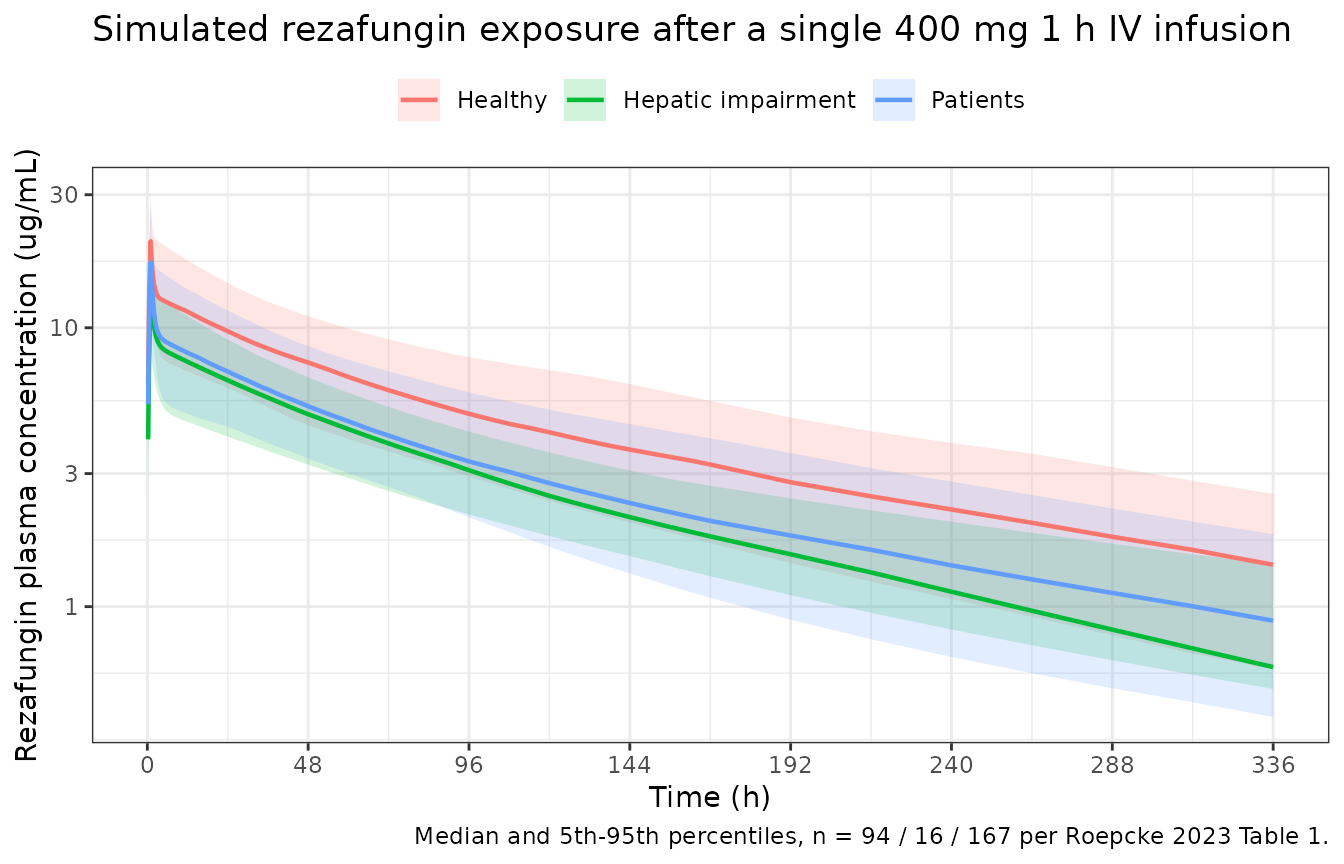

Figure 5 – weekly free AUC on the Phase 3 regimen

Roepcke 2023 Figure 5 shows boxplots of fAUC(0-168h) by week in patients given the ReSTORE regimen: 400 mg in week 1 followed by 200 mg weekly for three further weeks. Free concentrations use the 2.6% free fraction the paper adopted (Materials and Methods, target-attainment section).

set.seed(20230730)

n_pta <- 200L   # 200-per-arm cap; Roepcke 2023 used 100 x 1,000 virtual patients
pta_subjects <- make_subjects(
  cohort = "Patients", n = n_pta, dis_healthy = 0L,
  bsa_mean = 1.86, bsa_sd = 0.30, bsa_lo = 1.2, bsa_hi = 2.7,
  alb_mean = 2.63, alb_sd = 0.66, alb_lo = 1.2, alb_hi = 4.6,
  id_offset = 0L
)

dose_times <- c(0, 168, 336, 504)          # weekly
dose_amts  <- c(400, 200, 200, 200)        # 400 mg LD then 200 mg weekly

pta_dose_rows <- pta_subjects |>
  tidyr::expand_grid(tibble(time = dose_times, amt = dose_amts)) |>
  mutate(evid = 1L, cmt = "central", rate = amt / infusion_h)

week_offsets <- c(0, 0.25, 0.5, 0.75, 1, 1.5, 2, 3, 4, 6, 8, 12,
                  24, 48, 72, 96, 120, 144, 168)
pta_obs_times <- sort(unique(as.vector(outer(week_offsets, dose_times, `+`))))
pta_obs_times <- pta_obs_times[pta_obs_times <= 672]

pta_obs_rows <- pta_subjects |>
  tidyr::expand_grid(time = pta_obs_times) |>
  mutate(evid = 0L, amt = 0, cmt = "central", rate = 0)

pta_events <- bind_rows(pta_dose_rows, pta_obs_rows) |>
  arrange(id, time, desc(evid))

sim_pta <- rxode2::rxSolve(
  mod, events = pta_events, keep = c("cohort", "DIS_HEALTHY", "BSA", "ALB")
) |> as.data.frame()
stopifnot(dplyr::n_distinct(sim_pta$id) == n_pta)

# Guard against the same omega-reuse trap in the other direction: a
# population solve that follows a zeroRe() solve can silently come back
# without IIV. Individual CL should carry roughly the published 30.5 %CV.
cl_i <- vapply(split(sim_pta$cl, sim_pta$id), function(z) z[1], numeric(1))
stopifnot(stats::sd(cl_i) / mean(cl_i) > 0.15)

f_unbound <- 0.026   # Roepcke 2023: 2.6% free fraction (97.4% protein bound)

pta_nca <- sim_pta |>
  dplyr::filter(!is.na(Cc)) |>
  dplyr::select(id, time, Cc, cohort) |>
  dplyr::distinct(id, cohort, time, .keep_all = TRUE) |>
  arrange(id, time)

pta_conc <- PKNCA::PKNCAconc(pta_nca, Cc ~ time | cohort + id)
pta_dose <- PKNCA::PKNCAdose(
  pta_events |> dplyr::filter(evid == 1) |> dplyr::select(id, time, amt, cohort),
  amt ~ time | cohort + id
)

weekly_intervals <- data.frame(
  start   = dose_times,
  end     = dose_times + 168,
  auclast = TRUE
)

weekly_res <- PKNCA::pk.nca(
  PKNCA::PKNCAdata(pta_conc, pta_dose, intervals = weekly_intervals)
)

weekly <- as.data.frame(weekly_res) |>
  dplyr::filter(PPTESTCD == "auclast") |>
  mutate(
    week  = factor(match(start, dose_times), labels = paste("Week", 1:4)),
    fAUC  = PPORRES * f_unbound
  )

# Replicates Figure 5 of Roepcke 2023: fAUC(0-168h) by week, 400 mg week 1
# then 200 mg weekly. Reference lines are the Table 4 stasis fAUC/MIC
# targets evaluated at MIC = 0.25 ug/mL (see note below the figure).
mic_ref <- 0.25
targets <- tibble::tribble(
  ~species,             ~stasis, ~one_log,
  "C. albicans",        20.5,    37.2,
  "C. glabrata",         0.5,     2.94,
  "C. parapsilosis",    18.2,    NA_real_,
  "C. auris",           12.1,    38.4,
  "C. tropicalis",      86.5,   148.9,
  "C. dubliniensis",    35.1,   228.3
)

ggplot(weekly, aes(week, fAUC)) +
  geom_boxplot(fill = "grey85", outlier.size = 0.6) +
  geom_hline(
    data = targets |> mutate(y = stasis * mic_ref),
    aes(yintercept = y, colour = species), linetype = "dashed"
  ) +
  scale_y_log10() +
  labs(
    x = NULL, y = expression(italic(f) * "AUC"[0-168*h] ~ "(ug*h/mL)"),
    colour = "Stasis target at MIC 0.25 ug/mL",
    title = "Free weekly rezafungin AUC on the ReSTORE regimen",
    caption = paste(
      "Replicates Figure 5 of Roepcke 2023 (400 mg week 1, then 200 mg",
      "weekly). n = 200 simulated patients."
    )
  ) +
  theme_bw() +
  theme(legend.position = "right")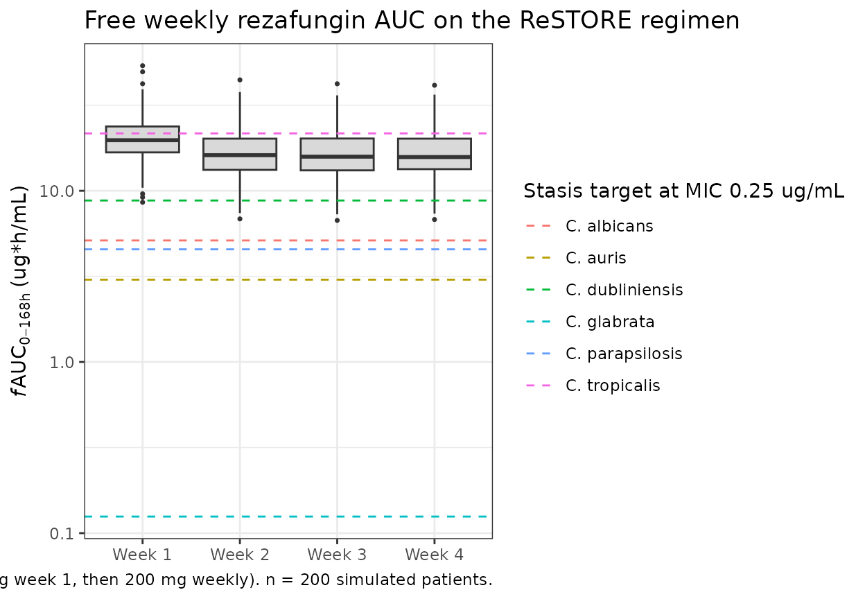

Roepcke 2023 draws its Figure 5 reference lines at the fAUC needed for stasis at each species’ MIC90; the MIC90 values live in the Figure 4 bar charts and are not tabulated, so the lines above are drawn instead at a single common MIC of 0.25 ug/mL, the value the paper quotes as the C. albicans and C. auris breakpoint. The figure reproduces the paper’s qualitative message: week-1 exposure (400 mg) is roughly twice the steady 200 mg weekly exposure, and weeks 2-4 are stable.

Figure 4 – probability of PK/PD target attainment

Roepcke 2023 Figure 4 reports the probability of attaining the nonclinical fAUC(0-168h)/MIC targets of Table 4 after the 400 mg day-1 dose.

The comparison has to be posed carefully. The paper defines its breakpoint as “the highest clinically relevant MIC value with a probability of PK/PD target attainment of at least 0.9” – the search is capped by the observed surveillance MIC distribution drawn as the bars of Figure 4, which is not tabulated anywhere in the article. The published breakpoints are therefore a lower bound on the PTA crossing point, not the crossing point itself, and a simulated crossing that lands above the published breakpoint is agreement, not disagreement. The testable claim is the one the paper’s Results actually makes – “the simulated probabilities of target attainment … were >90% at MIC values <= x” – so the check below evaluates simulated PTA at each published MIC and asks whether it clears 90%.

fauc_wk1 <- weekly |> dplyr::filter(week == "Week 1") |> dplyr::pull(fAUC)

targets_long <- targets |>
  tidyr::pivot_longer(c(stasis, one_log), names_to = "target", values_to = "ratio") |>
  dplyr::filter(!is.na(ratio)) |>
  mutate(target = ifelse(target == "stasis", "Stasis", "1-log drop"))

pta_of <- function(ratio, mic) mapply(function(r, m) mean(fauc_wk1 / m >= r), ratio, mic)

# MICs quoted in Roepcke 2023 Results, "Target attainment simulations".
# The paper writes 0.06 for the CLSI doubling-series value 0.0625.
published_bp <- tibble::tribble(
  ~species,          ~target,      ~mic_reported, ~mic_clsi,
  "C. albicans",     "Stasis",     "0.25",        0.25,
  "C. albicans",     "1-log drop", "0.25",        0.25,
  "C. glabrata",     "Stasis",     "4",           4,
  "C. glabrata",     "1-log drop", "4",           4,
  "C. parapsilosis", "Stasis",     "0.5",         0.5,
  "C. auris",        "Stasis",     "0.25",        0.25,
  "C. auris",        "1-log drop", "0.25",        0.25,
  "C. tropicalis",   "Stasis",     "0.06",        0.0625,
  "C. tropicalis",   "1-log drop", "0.06",        0.0625,
  "C. dubliniensis", "Stasis",     "0.06",        0.0625,
  "C. dubliniensis", "1-log drop", "0.06",        0.0625
)

mic_grid <- 2^seq(-7, 4)   # 0.0078 to 16 ug/mL

pta <- tidyr::expand_grid(targets_long, mic = mic_grid) |>
  mutate(pta = pta_of(ratio, mic))

crossing <- pta |>
  dplyr::filter(pta >= 0.9) |>
  group_by(species, target) |>
  summarise(crossing = max(mic), .groups = "drop")

published_bp |>
  left_join(targets_long, by = c("species", "target")) |>
  mutate(`Simulated PTA at that MIC` = pta_of(ratio, mic_clsi)) |>
  left_join(crossing, by = c("species", "target")) |>
  mutate(
    `Clears 90%?`                = ifelse(`Simulated PTA at that MIC` >= 0.9, "yes", "NO"),
    `Simulated PTA at that MIC`  = paste0(round(100 * `Simulated PTA at that MIC`), "%")
  ) |>
  dplyr::select(
    "Species" = species, "PK/PD target" = target,
    "Roepcke 2023 MIC (ug/mL)" = mic_reported,
    "Simulated PTA at that MIC", "Clears 90%?",
    "Simulated PTA >= 0.9 up to (ug/mL)" = crossing
  ) |>
  knitr::kable(
    caption = paste(
      "Target attainment after a single 400 mg dose. The paper claims PTA",
      ">90% at each listed MIC; the last column is the uncapped simulated",
      "crossing point, which may legitimately exceed the published",
      "breakpoint because the paper caps its search at the highest",
      "clinically relevant MIC."
    )
  )

Target attainment after a single 400 mg dose. The paper claims PTA >90% at each listed MIC; the last column is the uncapped simulated crossing point, which may legitimately exceed the published breakpoint because the paper caps its search at the highest clinically relevant MIC.
Species	PK/PD target	Roepcke 2023 MIC (ug/mL)	Simulated PTA at that MIC	Clears 90%?	Simulated PTA >= 0.9 up to (ug/mL)
C. albicans	Stasis	0.25	100%	yes	0.5000
C. albicans	1-log drop	0.25	99%	yes	0.2500
C. glabrata	Stasis	4	100%	yes	16.0000
C. glabrata	1-log drop	4	97%	yes	4.0000
C. parapsilosis	Stasis	0.5	100%	yes	0.5000
C. auris	Stasis	0.25	100%	yes	1.0000
C. auris	1-log drop	0.25	99%	yes	0.2500
C. tropicalis	Stasis	0.06	100%	yes	0.1250
C. tropicalis	1-log drop	0.06	99%	yes	0.0625
C. dubliniensis	Stasis	0.06	100%	yes	0.2500
C. dubliniensis	1-log drop	0.06	90%	yes	0.0625

ggplot(pta, aes(mic, pta, colour = target)) +
  geom_line(linewidth = 0.7) +
  geom_point(size = 1) +
  geom_hline(yintercept = 0.9, linetype = "dotted") +
  scale_x_log10() +
  scale_y_continuous(labels = function(x) paste0(100 * x, "%"), limits = c(0, 1)) +
  facet_wrap(~species) +
  labs(
    x = "MIC (ug/mL)", y = "Probability of target attainment",
    colour = NULL,
    title = "Replicates Figure 4 of Roepcke 2023",
    caption = paste(
      "PTA of the Table 4 nonclinical fAUC(0-168h)/MIC targets after the",
      "400 mg day-1 dose; dotted line = 0.9. n = 200 simulated patients."
    )
  ) +
  theme_bw() +
  theme(legend.position = "top")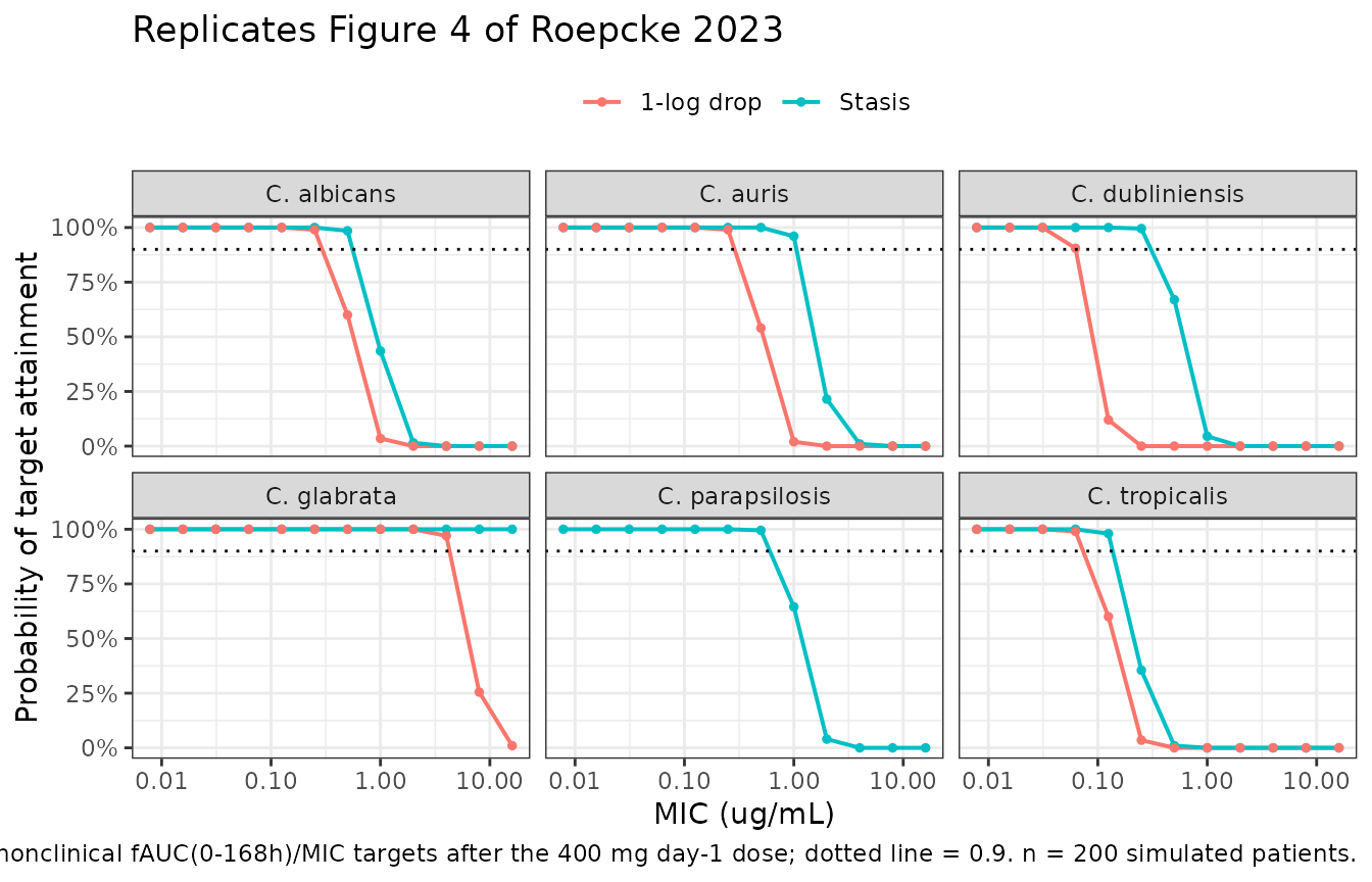

Assumptions and deviations

BSA and albumin distributions are reconstructed, not observed. The virtual cohorts sample both covariates from independent normal distributions matched to the Roepcke 2023 Table 1 per-stratum mean and SD and clamped to the published per-stratum range. The real cohort’s BSA and albumin are correlated with each other and with health status, and both are skewed (Table 1 medians differ from means, particularly for the patient stratum). Simulated exposure spread is therefore an approximation of, not a reproduction of, the published spread.
The hepatic-impairment stratum agrees least well, as expected. Its simulated Cmax, AUC, and half-life sit 13-19% from Roepcke 2023 Table 3 while the healthy and patient strata land within about 6%. That stratum has only 16 subjects and the widest relative gap between the Table 1 mean and median (BSA 2.13 vs 2.10 m^2; albumin 3.71 vs 3.70 g/dL with SD 0.60), so a symmetric normal draw around the mean reproduces its covariate distribution least faithfully. All 12 comparisons remain inside the 20% tolerance.
BSA formula is unspecified in the source. Roepcke 2023 tabulates BSA as a baseline characteristic but never states whether it was computed by DuBois, Mosteller, or Haycock. The model consumes BSA as a supplied covariate column, so the choice does not affect the packaged model; it does affect how a user should derive BSA for their own data.
Sign of the three covariate coefficients comes from the Table 2 footnote-a equations, not the Table 2 body. Table 2 lists Exponent of (ALB/3.2) for V23 as 0.708 and the two disease-state shifts as 0.276 and 0.222, all unsigned; footnote a prints them as -0.708, 1 + (-0.276) x I_healthy, and 1 + (-0.222) x I_healthy. The negative orientation is independently corroborated by Table 3 (the low-albumin patient stratum has the larger Vss) and by the Results sentence “healthy subjects had a 27.6% lower CL”.
Vss is V1 + 2 x V23. Table 3 footnote b defines the individual Vss as the sum of the central and the peripheral volumes. Because Roepcke 2023 collapsed V2 and V3 into one shared parameter, both peripheral compartments contribute V23, so Vss = V1 + 2 x V23. Using V1 + V23 reproduces only about two-thirds of the published Vss and is wrong.
Cohort size for target attainment is 200, not 100,000. Roepcke 2023 simulated 100 trials of 1,000 virtual patients each by resampling covariate vectors from the observed Phase 2 / Phase 3 distributions. This vignette uses 200 simulated patients with parametrically sampled covariates, per the 200-per-arm cap. PTA estimates therefore carry Monte Carlo noise of roughly +/-3 percentage points, which can move a crossing point by one doubling dilution near the 0.9 threshold.
The published MIC breakpoints cannot be reproduced as crossing points. Roepcke 2023 defines the breakpoint as the highest clinically relevant MIC with PTA >= 0.9, capping the search at the observed surveillance MIC distribution plotted as the bars of Figure 4. Those MIC distributions are not tabulated in the article or its supplement, so the cap cannot be applied here. The published breakpoints are consequently lower bounds, and the validation above tests the paper’s actual claim (PTA >= 90% at each reported MIC) rather than equality of crossing points. The uncapped simulated crossing exceeds the published breakpoint for several stasis targets, which is consistent with, not contradictory to, the paper.
Figure 5 reference lines use a single MIC of 0.25 ug/mL. The paper’s reference lines are drawn at each species’ MIC90, which appears only in the Figure 4 bar charts and is not tabulated, so it could not be transcribed.
The Phase 2 STRIVE Group 1 regimen (400 mg weekly) is not simulated. Only the ReSTORE / STRIVE Group 2 regimen (400 mg loading dose then 200 mg weekly) is reproduced, matching the regimen Roepcke 2023 carried into its target-attainment analysis.
Covariates screened but not retained (age, weight, BMI, sex, serum creatinine, creatinine clearance, ALT, AST, APACHE score) are documented in the model file’s covariatesDataExcluded list for provenance. They are not referenced in model() because Roepcke 2023 did not retain them.
No non-paper-derived parameter values. Every value in ini() comes from Roepcke 2023 Table 2 or its footnote a; no author correspondence, figure digitisation, or upstream-model carry-over was needed.