Levonorgestrel and ethinyl estradiol transdermal system (Stanczyk 2022)
Source:vignettes/articles/Stanczyk_2022_levonorgestrel_ethinylestradiol.Rmd
Stanczyk_2022_levonorgestrel_ethinylestradiol.RmdModel and source
- Citation: Stanczyk FZ, Archer DF, Lohmer LRL, Pirone J, Previtera M, Korner P. Extended regimen of a levonorgestrel/ethinyl estradiol transdermal delivery system: Predicted serum hormone levels using a population pharmacokinetic model. PLoS ONE. 2022;17(12):e0279640. doi:10.1371/journal.pone.0279640
- Levonorgestrel model: One-compartment population PK model for
levonorgestrel (LNG) delivered by the once-weekly levonorgestrel/ethinyl
estradiol transdermal delivery system (TDS) in healthy women (Stanczyk
2022). Each 7-day patch splits its bioavailable dose between a short
zero-order infusion into a first-order absorption depot (fraction Frel)
and a zero-order input directly into the central compartment over the
168-h wear period (fraction 1 - Frel). Overall bioavailability F = 27%
is fixed. Clearance and volume are lower from the third consecutive
weekly patch onwards (multipliers 0.87 and 0.85). Dose each patch as TWO
records of the patch LNG content (2600 ug): one to
depotwithrate = -2(modelled duration D1) and one tocentralwith an explicitdur = 168, which equals the model’s fixed D2 and avoids an rxode2 5.1.8 mis-solve of back-to-back modelled-duration infusions when CYCLE changes on the dose row (see vignette); f() splits the content between the two routes. - Ethinyl estradiol model: One-compartment population PK model for
ethinyl estradiol (EE) delivered by the once-weekly
levonorgestrel/ethinyl estradiol transdermal delivery system (TDS) in
healthy women (Stanczyk 2022). Each 7-day patch splits its bioavailable
dose between a zero-order input directly into the central compartment
over the 168-h wear period (fraction Frel) and a bolus into a
first-order absorption depot (fraction 1 - Frel). Overall
bioavailability F = 30% is fixed. Dose each patch as TWO records of the
patch EE content (2300 ug), one to
centralwithrate = -2and one todepot; f() splits the content between the two routes. - Article: https://doi.org/10.1371/journal.pone.0279640
- Supporting information (S1-S4 Tables, S1-S2 Figs): https://journals.plos.org/plosone/article?id=10.1371/journal.pone.0279640#sec014
Stanczyk 2022 fitted two separate one-compartment population PK
models in Phoenix NLME 8.1, one for levonorgestrel (LNG) and one for
ethinyl estradiol (EE), to cycle-2 data from women wearing the
once-weekly LNG/EE transdermal delivery system (TDS). The models were
then used to simulate a 12-week extended regimen and to show that weeks
3 and 12 give the same exposure. The two models are packaged as
Stanczyk_2022_levonorgestrel and
Stanczyk_2022_ethinylestradiol. The final parameter
estimates are printed only in the supporting information (S1 and S2
Tables); the simulated concentrations at each nominal time point are in
S3 and S4 Tables.
Population
The source study was ATI-CL14 (NCT01243580), a phase 1, open-label, randomized, single-centre trial run in 2009 in 36 healthy, normotensive, nonsmoking women aged 18 to 45 years with a BMI of 18 to 32 kg/m^2 and 24- to 35-day menstrual intervals. The popPK models used only the cycle-2 data of the 18 women who wore the TDS in cycles 1 and 2. Samples were taken before patch application and at 6, 12, 24, 48, 72, 120, 144 and 168 h in weeks 1 and 3, plus 174 to 240 h after the third patch (23 samples per woman). Each patch contains 2.6 mg LNG and 2.3 mg EE and nominally delivers 120 ug/day LNG and 30 ug/day EE. No covariate analysis was performed and no demographic table for the 18 women is given (Methods, “Study design” and “PopPK models”).
Source trace
| Quantity | Value | Source |
|---|---|---|
| EE structure: zero-order input into central over 168 h (fraction Frel) plus first-order depot (1 - Frel) | – | Methods, “EE popPK models” |
| EE V | 2490 L | S1 Table |
| EE CL | 107 L/h | S1 Table |
| EE Ka | 0.0204 1/h | S1 Table |
| EE Frel (zero-order route) | 0.732 | S1 Table |
| EE F | 0.30 (fixed) | S1 Table; Methods |
| EE IIV V / CL / Ka | 43.4 / 34.6 / 53.1 % CV | S1 Table |
| EE residual error | 26.9 % proportional | S1 Table and footnote |
| LNG structure: depot infused over D1 (fraction Frel) with first-order absorption, plus zero-order input into central over 168 h (1 - Frel) | – | Methods, “LNG popPK model” |
| LNG V, CL (patches 1-2) | 163 L, 2.46 L/h | S2 Table |
| LNG week-3 effect on V, CL | 85.0 %, 87.0 % (multipliers 0.85, 0.87) | S2 Table; reading checked below |
| LNG Ka | 0.0281 1/h | S2 Table |
| LNG Frel (first-order route) | 0.378 | S2 Table |
| LNG F | 0.27 (fixed) | S2 Table; Methods |
| LNG D1 (depot infusion duration) | 0.5 h, back-solved | not printed; S4 Table week 1 (see below) |
| LNG IIV V / CL / Frel | 38.9 / 44.4 / 23.5 % CV | S2 Table |
| LNG residual error | proportional SD 0.206, additive SD 0.0860 ug/L | S2 Table and footnote |
| Dose per patch | 2600 ug LNG, 2300 ug EE | Methods, “Extended regimen simulations” |
Virtual cohort and extended-regimen simulation
The paper simulated 1000 women wearing 12 consecutive weekly patches
and summarised weeks 1, 3 and 12. Here 200 women are simulated per drug
with the full between-subject variability and without residual error, as
in the paper. Each patch is two dose records of the patch content, one
to depot and one to central.
The central record is given an explicit dur = 168 rather
than rate = -2. The model fixes the central input duration
at 168 h, so the two are the same model, but rxode2 5.1.8 mis-handles a
modelled-duration (rate = -2) infusion that ends at the
instant the next one starts when a covariate changes on the new dose
row, as CYCLE does here: the weekly central input is then
delivered almost at once. An explicit duration is unaffected (checked
below against the closed-form steady-state AUC). The LNG depot record
keeps rate = -2 so the model’s 0.5 h
dur(depot) applies; the EE depot record is a bolus.
CYCLE is the number of the patch being worn. The
observation that closes week w (and is time 0 of week w +
1) is given the CYCLE of week w and placed before the next
patch, so it is the pre-dose value the paper tabulates as “time 0”.
n_sub <- 200
n_patch <- 12
dose_lng <- 2600 # ug LNG per patch
dose_ee <- 2300 # ug EE per patch
weeks_obs <- c(1, 3, 12)

dose_rows <- tidyr::expand_grid(patch = seq_len(n_patch), cmt = c("depot", "central")) |>
  mutate(time = 168 * (patch - 1), evid = 1L, CYCLE = patch)

obs_rows <- tidyr::expand_grid(week = weeks_obs, rt = 0:168) |>
  mutate(
    time = 168 * (week - 1) + rt,
    evid = 0L,
    cmt = "central",
    rate = 0,
    dur = 0,
    # Time 0 of a week is the pre-dose value, still under the previous patch.
    CYCLE = ifelse(rt == 0, pmax(week - 1, 1), week)
  )

make_events <- function(amt, depot_rate) {
  doses <- dose_rows |>
    mutate(
      amt = amt,
      rate = ifelse(cmt == "depot", depot_rate, 0),
      dur = ifelse(cmt == "central", 168, 0)
    )
  one <- bind_rows(doses, mutate(obs_rows, amt = 0)) |>
    # observation before dose at a shared time
    arrange(time, evid) |>
    select(time, evid, amt, cmt, rate, dur, CYCLE)
  tidyr::expand_grid(id = seq_len(n_sub), one) |>
    select(id, time, evid, amt, cmt, rate, dur, CYCLE)
}
ev_lng <- make_events(dose_lng, depot_rate = -2)
ev_ee <- make_events(dose_ee, depot_rate = 0)
mod_lng <- readModelDb("Stanczyk_2022_levonorgestrel")
mod_ee <- readModelDb("Stanczyk_2022_ethinylestradiol")

rxode2::rxSetSeed(20221227)
sim_lng <- rxode2::rxSolve(mod_lng, ev_lng, returnType = "data.frame")
#> ℹ parameter labels from comments will be replaced by 'label()'
rxode2::rxSetSeed(20221228)
sim_ee <- rxode2::rxSolve(mod_ee, ev_ee, returnType = "data.frame")
#> ℹ parameter labels from comments will be replaced by 'label()'

week_of <- function(time) {
  # Week 1 is [0, 168]; week 3 is [336, 504]; week 12 is [1848, 2016].
  w <- rep(NA_real_, length(time))
  for (wk in weeks_obs) {
    w[time >= 168 * (wk - 1) & time <= 168 * wk & is.na(w)] <- wk
  }
  w
}

conc <- bind_rows(
  sim_lng |> mutate(drug = "LNG"),
  sim_ee |> mutate(drug = "EE")
) |>
  select(id, time, drug, Cc) |>
  mutate(week = week_of(time), rt = time - 168 * (week - 1)) |>
  filter(!is.na(week)) |>
  # each solve returns one row per observation record
  distinct(id, drug, week, rt, .keep_all = TRUE) |>
  mutate(conc_pg = 1000 * Cc) # ng/mL -> pg/mL
stopifnot(!anyNA(conc$Cc))
Cc is the individual prediction, i.e. without residual
error, matching the paper.
Back-solving the LNG depot infusion duration
The Methods state that the duration of the zero-order infusion into the LNG dosing compartment “was estimated by the model”, but S2 Table does not print it. Every other LNG parameter is printed, so the duration was back-solved from the paper’s own week-1 simulation (S4 Table). Only the earliest time points depend on it: by 24 h the depot has received its whole dose for any duration of a few hours. The table below shows the typical-value concentrations for a range of durations; the shortest durations fit the S4 Table 6-h and 12-h values best. The maintainers fitted the duration by least squares to the S4 Table week-1 means and medians at 6 and 12 h with a 4000-subject simulation, scanning 0.1 to 2 h; the optimum was 0.5 h, which is what the model ships. Any duration up to about 2 h stays within 5% of those four values, so the exact value hardly matters, but durations of 8 h or more do not fit.
ev_wk1 <- rxode2::et(amt = dose_lng, cmt = "depot", rate = -2) |>
  rxode2::et(amt = dose_lng, cmt = "central", rate = -2) |>
  rxode2::et(c(6, 12, 24, 48)) |>
  as.data.frame() |>
  mutate(CYCLE = 1)
d1_scan <- lapply(c(0.05, 0.5, 2, 8, 24), function(d1) {
  s <- rxode2::rxSolve(rxode2::zeroRe(mod_lng), ev_wk1,
    params = c(ld1 = log(d1)), returnType = "data.frame")
  data.frame(d1 = d1, time = s$time, conc = round(1000 * s$Cc))
}) |>
  bind_rows() |>
  tidyr::pivot_wider(names_from = time, values_from = conc, names_prefix = "t")
#> ℹ parameter labels from comments will be replaced by 'label()'
#> ℹ omega/sigma items treated as zero: 'etalvc', 'etalcl', 'etalfrel'
#> ℹ parameter labels from comments will be replaced by 'label()'
#> ℹ omega/sigma items treated as zero: 'etalvc', 'etalcl', 'etalfrel'
#> ℹ parameter labels from comments will be replaced by 'label()'
#> ℹ omega/sigma items treated as zero: 'etalvc', 'etalcl', 'etalfrel'
#> ℹ parameter labels from comments will be replaced by 'label()'
#> ℹ omega/sigma items treated as zero: 'etalvc', 'etalcl', 'etalfrel'
#> ℹ parameter labels from comments will be replaced by 'label()'
#> ℹ omega/sigma items treated as zero: 'etalvc', 'etalcl', 'etalfrel'
d1_scan |>
  dplyr::rename(
    "Depot infusion duration (h)" = d1,
    "6 h" = t6, "12 h" = t12, "24 h" = t24, "48 h" = t48
  ) |>
knitr::kable(caption = "Typical-value LNG concentration (pg/mL) in week 1 by depot infusion duration. S4 Table week-1 medians: 330, 591, 949 and 1260 pg/mL.")| Depot infusion duration (h) | 6 h | 12 h | 24 h | 48 h |
|---|---|---|---|---|
| 0.05 | 332 | 598 | 977 | 1336 |
| 0.50 | 324 | 592 | 974 | 1336 |
| 2.00 | 297 | 572 | 964 | 1336 |
| 8.00 | 186 | 479 | 914 | 1332 |
| 24.00 | 123 | 291 | 713 | 1295 |
wk1_early <- conc |>
  filter(drug == "LNG", week == 1, rt %in% c(6, 12)) |>
  group_by(rt) |>
  summarise(mean = mean(conc_pg), median = median(conc_pg), .groups = "drop")
paper_wk1 <- data.frame(rt = c(6, 12), mean = c(357, 632), median = c(330, 591))
wk1_early
#> # A tibble: 2 × 3
#>      rt  mean median
#>   <dbl> <dbl>  <dbl>
#> 1     6  355.   331.
#> 2    12  641.   593.
stopifnot(
  # The 0.5 h duration reproduces the S4 Table early week-1 values; an 8 h
  # duration would put the 6 h median about 40% low.
  all(abs(wk1_early$median / paper_wk1$median - 1) < 0.15),
  all(abs(wk1_early$mean / paper_wk1$mean - 1) < 0.15)
)
Reading of the LNG week-3 effect
S2 Table prints “Week 3 effect on volume (%) 85.0” and “Week 3 effect on clearance (%) 87.0”. These are read as multipliers: from week 3, V = 0.85 x 163 L and CL = 0.87 x 2.46 L/h. Two checks support this reading:
- At steady state the weekly AUC equals F x dose / CL. With CL = 0.87 x 2.46 L/h this is 0.27 x 2600 / 2.14 = 328 hng/mL, against the paper’s week-12 geometric mean AUC(0-168) of 326 hng/mL (Table 3). The other readings, 1.87 x CL or 0.13 x CL, give 153 or 2190 h*ng/mL.
- The effect has to start at the third patch, not the second. The S4 Table week-3 pre-dose mean (1410 pg/mL) is the end of week 2 under the reference volume; if the lower volume applied already in week 2, the pre-dose mean would be about 1640 pg/mL. The paper’s extended-regimen simulation applies the week-3 values to every later patch, as the week-12 rows show.
typ_lng <- rxode2::zeroRe(mod_lng)
#> ℹ parameter labels from comments will be replaced by 'label()'
ev_typ <- ev_lng |> filter(id == 1)
s_typ <- rxode2::rxSolve(typ_lng, ev_typ, returnType = "data.frame") |>
  mutate(week = week_of(time), rt = time - 168 * (week - 1)) |>
  filter(week == 12) |>
  distinct(rt, .keep_all = TRUE)
#> ℹ omega/sigma items treated as zero: 'etalvc', 'etalcl', 'etalfrel'
auc_wk12_typ <- sum(diff(s_typ$rt) * (head(s_typ$Cc, -1) + tail(s_typ$Cc, -1)) / 2)
auc_wk12_ss <- 0.27 * dose_lng / (0.87 * 2.46)
c(simulated = auc_wk12_typ, closed_form = auc_wk12_ss)
#>   simulated closed_form
#>    328.0067    328.0067
stopifnot(
  # Steady-state identity on the typical subject: the same parameters on both
  # sides, so only trapezoid and carry-over error separate them.
  abs(auc_wk12_typ / auc_wk12_ss - 1) < 0.02
)

predose_wk3 <- conc |> filter(drug == "LNG", week == 3, rt == 0)
c(mean = mean(predose_wk3$conc_pg), median = median(predose_wk3$conc_pg))
#>     mean   median
#> 1460.219 1340.394
stopifnot(
  # S4 Table week-3 time-0 median 1270 pg/mL; the week-2 onset reading gives
  # about 1490.
  abs(median(predose_wk3$conc_pg) / 1270 - 1) < 0.10
)
Replicating Figure 1 and S3/S4 Tables
mean_prof <- conc |>
  group_by(drug, week, rt) |>
  summarise(mean_conc = mean(conc_pg), .groups = "drop") |>
  mutate(
    week = factor(paste("Week", week), levels = paste("Week", weeks_obs)),
    drug = factor(drug, levels = c("EE", "LNG"))
  )
ggplot(mean_prof, aes(rt, mean_conc, colour = week)) +
  geom_line() +
  facet_wrap(~drug, scales = "free_y") +
  scale_x_continuous(breaks = seq(0, 168, 24)) +
  labs(
    x = "Time since patch application (h)",
    y = "Mean concentration (pg/mL)",
    colour = NULL,
    caption = "Replicates Figure 1 of Stanczyk 2022 (A: EE, B: LNG)."
  ) +
  theme_bw()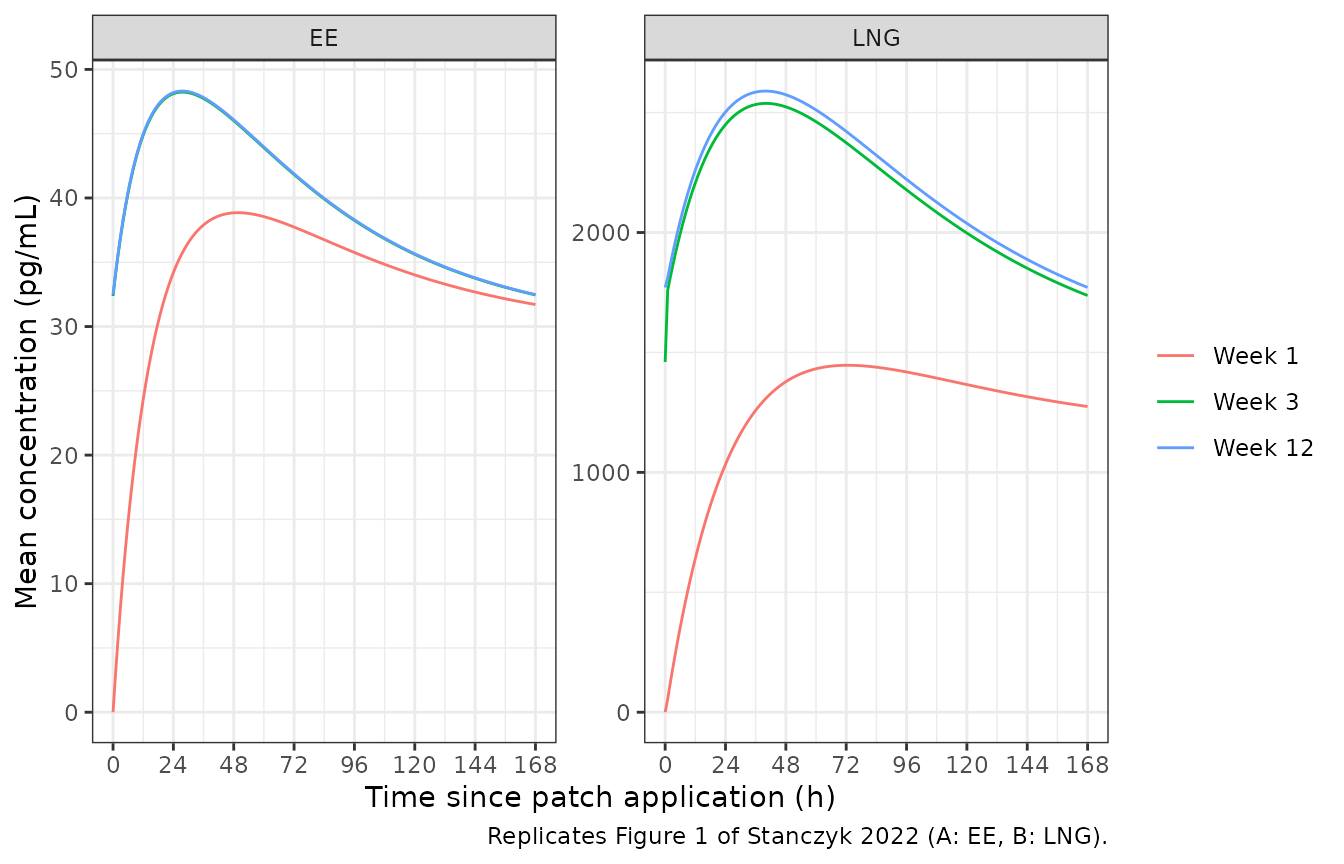
nominal <- c(0, 6, 12, 24, 48, 72, 120, 144, 168)
paper_s3s4 <- bind_rows(
  data.frame(
    drug = "EE", week = rep(weeks_obs, each = 9), rt = nominal,
    paper_mean = c(
      0, 15.4, 25.2, 35.2, 39.4, 38.1, 34.3, 33.0, 32.1,
      32.8, 41.4, 46.1, 49.4, 46.8, 42.4, 36.0, 34.2, 32.9,
      33.0, 41.5, 46.2, 49.5, 46.9, 42.4, 36.1, 34.2, 33.0
    ),
    paper_median = c(
      0, 14.1, 23.5, 33.5, 37.7, 36.0, 31.9, 30.7, 29.8,
      30.3, 38.6, 43.5, 46.9, 43.7, 39.0, 33.3, 31.6, 30.3,
      30.4, 38.6, 43.5, 47.0, 43.7, 39.1, 33.4, 31.6, 30.4
    )
  ),
  data.frame(
    drug = "LNG", week = rep(weeks_obs, each = 9), rt = nominal,
    paper_mean = c(
      0, 357, 632, 1000, 1320, 1380, 1310, 1260, 1220,
      1410, 1940, 2140, 2370, 2430, 2280, 1930, 1780, 1680,
      1700, 1980, 2190, 2410, 2470, 2320, 1950, 1810, 1700
    ),
    paper_median = c(
      0, 330, 591, 949, 1260, 1330, 1250, 1190, 1140,
      1270, 1770, 1970, 2200, 2250, 2100, 1730, 1590, 1480,
      1480, 1760, 1980, 2200, 2250, 2110, 1730, 1590, 1480
    )
  )
)

cmp_s3s4 <- conc |>
  filter(rt %in% nominal) |>
  group_by(drug, week, rt) |>
  summarise(sim_mean = mean(conc_pg), sim_median = median(conc_pg), .groups = "drop") |>
  inner_join(paper_s3s4, by = c("drug", "week", "rt")) |>
  mutate(pct_diff_mean = ifelse(paper_mean > 0, 100 * (sim_mean / paper_mean - 1), NA_real_))

cmp_s3s4 |>
  mutate(across(c(sim_mean, sim_median), ~ signif(.x, 3)), pct_diff_mean = round(pct_diff_mean, 1)) |>
  dplyr::rename(
    "Drug" = drug, "Week" = week, "Time (h)" = rt,
    "Simulated mean (pg/mL)" = sim_mean, "Paper mean (pg/mL)" = paper_mean,
    "Simulated median (pg/mL)" = sim_median, "Paper median (pg/mL)" = paper_median,
    "Mean % diff" = pct_diff_mean
  ) |>
knitr::kable(caption = "Simulated concentrations against S3 Table (EE) and S4 Table (LNG) of Stanczyk 2022.")| Drug | Week | Time (h) | Simulated mean (pg/mL) | Simulated median (pg/mL) | Paper mean (pg/mL) | Paper median (pg/mL) | Mean % diff |
|---|---|---|---|---|---|---|---|
| EE | 1 | 0 | 0.0 | 0.0 | 0.0 | 0.0 | NA |
| EE | 1 | 6 | 14.9 | 13.5 | 15.4 | 14.1 | -3.4 |
| EE | 1 | 12 | 24.3 | 22.2 | 25.2 | 23.5 | -3.4 |
| EE | 1 | 24 | 34.2 | 32.1 | 35.2 | 33.5 | -2.8 |
| EE | 1 | 48 | 38.8 | 36.9 | 39.4 | 37.7 | -1.4 |
| EE | 1 | 72 | 37.7 | 35.8 | 38.1 | 36.0 | -1.0 |
| EE | 1 | 120 | 34.0 | 31.3 | 34.3 | 31.9 | -0.8 |
| EE | 1 | 144 | 32.7 | 30.0 | 33.0 | 30.7 | -1.0 |
| EE | 1 | 168 | 31.7 | 29.0 | 32.1 | 29.8 | -1.2 |
| EE | 3 | 0 | 32.4 | 29.3 | 32.8 | 30.3 | -1.3 |
| EE | 3 | 6 | 40.4 | 37.4 | 41.4 | 38.6 | -2.4 |
| EE | 3 | 12 | 44.9 | 42.5 | 46.1 | 43.5 | -2.6 |
| EE | 3 | 24 | 48.1 | 45.5 | 49.4 | 46.9 | -2.6 |
| EE | 3 | 48 | 46.0 | 42.5 | 46.8 | 43.7 | -1.7 |
| EE | 3 | 72 | 41.8 | 38.0 | 42.4 | 39.0 | -1.4 |
| EE | 3 | 120 | 35.6 | 32.2 | 36.0 | 33.3 | -1.0 |
| EE | 3 | 144 | 33.8 | 30.6 | 34.2 | 31.6 | -1.3 |
| EE | 3 | 168 | 32.5 | 29.3 | 32.9 | 30.3 | -1.3 |
| EE | 12 | 0 | 32.5 | 29.3 | 33.0 | 30.4 | -1.6 |
| EE | 12 | 6 | 40.5 | 37.5 | 41.5 | 38.6 | -2.4 |
| EE | 12 | 12 | 45.0 | 42.5 | 46.2 | 43.5 | -2.6 |
| EE | 12 | 24 | 48.2 | 45.7 | 49.5 | 47.0 | -2.6 |
| EE | 12 | 48 | 46.1 | 42.5 | 46.9 | 43.7 | -1.7 |
| EE | 12 | 72 | 41.9 | 38.0 | 42.4 | 39.1 | -1.2 |
| EE | 12 | 120 | 35.7 | 32.2 | 36.1 | 33.4 | -1.2 |
| EE | 12 | 144 | 33.8 | 30.6 | 34.2 | 31.6 | -1.2 |
| EE | 12 | 168 | 32.5 | 29.3 | 33.0 | 30.4 | -1.6 |
| LNG | 1 | 0 | 0.0 | 0.0 | 0.0 | 0.0 | NA |
| LNG | 1 | 6 | 355.0 | 331.0 | 357.0 | 330.0 | -0.7 |
| LNG | 1 | 12 | 641.0 | 593.0 | 632.0 | 591.0 | 1.5 |
| LNG | 1 | 24 | 1030.0 | 978.0 | 1000.0 | 949.0 | 3.4 |
| LNG | 1 | 48 | 1380.0 | 1310.0 | 1320.0 | 1260.0 | 4.4 |
| LNG | 1 | 72 | 1450.0 | 1390.0 | 1380.0 | 1330.0 | 4.8 |
| LNG | 1 | 120 | 1370.0 | 1320.0 | 1310.0 | 1250.0 | 4.3 |
| LNG | 1 | 144 | 1320.0 | 1280.0 | 1260.0 | 1190.0 | 4.4 |
| LNG | 1 | 168 | 1270.0 | 1230.0 | 1220.0 | 1140.0 | 4.5 |
| LNG | 3 | 0 | 1460.0 | 1340.0 | 1410.0 | 1270.0 | 3.6 |
| LNG | 3 | 6 | 2000.0 | 1900.0 | 1940.0 | 1770.0 | 2.9 |
| LNG | 3 | 12 | 2210.0 | 2090.0 | 2140.0 | 1970.0 | 3.1 |
| LNG | 3 | 24 | 2450.0 | 2290.0 | 2370.0 | 2200.0 | 3.4 |
| LNG | 3 | 48 | 2520.0 | 2360.0 | 2430.0 | 2250.0 | 3.9 |
| LNG | 3 | 72 | 2370.0 | 2220.0 | 2280.0 | 2100.0 | 4.1 |
| LNG | 3 | 120 | 2000.0 | 1820.0 | 1930.0 | 1730.0 | 3.5 |
| LNG | 3 | 144 | 1850.0 | 1690.0 | 1780.0 | 1590.0 | 4.0 |
| LNG | 3 | 168 | 1740.0 | 1560.0 | 1680.0 | 1480.0 | 3.4 |
| LNG | 12 | 0 | 1770.0 | 1560.0 | 1700.0 | 1480.0 | 4.2 |
| LNG | 12 | 6 | 2050.0 | 1870.0 | 1980.0 | 1760.0 | 3.5 |
| LNG | 12 | 12 | 2260.0 | 2090.0 | 2190.0 | 1980.0 | 3.2 |
| LNG | 12 | 24 | 2500.0 | 2300.0 | 2410.0 | 2200.0 | 3.8 |
| LNG | 12 | 48 | 2570.0 | 2380.0 | 2470.0 | 2250.0 | 4.2 |
| LNG | 12 | 72 | 2420.0 | 2230.0 | 2320.0 | 2110.0 | 4.4 |
| LNG | 12 | 120 | 2040.0 | 1840.0 | 1950.0 | 1730.0 | 4.5 |
| LNG | 12 | 144 | 1890.0 | 1690.0 | 1810.0 | 1590.0 | 4.3 |
| LNG | 12 | 168 | 1770.0 | 1560.0 | 1700.0 | 1480.0 | 4.2 |
NCA with PKNCA
AUC(0-168), Cmax and Css(0-168) = AUC(0-168)/168 (PKNCA
cav) are computed per woman and week with PKNCA, using the
paper’s linear-up/log-down rule. Css(48-168) is the average over 48 to
168 h.
nca_conc <- conc |>
  mutate(treatment = paste0(drug, " week ", week)) |>
  select(id, treatment, drug, week, rt, conc_ng = Cc)

conc_obj <- PKNCA::PKNCAconc(nca_conc, conc_ng ~ rt | treatment + id)
intervals <- data.frame(
  start = c(0, 48),
  end = c(168, 168),
  cmax = c(TRUE, FALSE),
  auclast = c(TRUE, FALSE),
  cav = c(TRUE, TRUE)
)
nca_data <- PKNCA::PKNCAdata(conc_obj, intervals = intervals,
  options = list(auc.method = "lin up/log down"))
nca_res <- PKNCA::pk.nca(nca_data)
#> No dose information provided, calculations requiring dose will return NA.

nca_wide <- as.data.frame(nca_res) |>
  # PKNCA also reports the dependencies it computed (e.g. AUC for 48-168 h)
  filter(
    (start == 0 & PPTESTCD %in% c("cmax", "auclast", "cav")) |
      (start == 48 & PPTESTCD == "cav")
  ) |>
  mutate(PPTESTCD = ifelse(PPTESTCD == "cav" & start == 48, "cav48", PPTESTCD)) |>
  select(treatment, id, PPTESTCD, PPORRES) |>
  tidyr::pivot_wider(names_from = PPTESTCD, values_from = PPORRES)

geo <- function(x) exp(mean(log(x)))
nca_geo <- nca_wide |>
  group_by(treatment) |>
  summarise(
    cmax = geo(cmax) * 1000, auclast = geo(auclast),
    cav = geo(cav) * 1000, cav48 = geo(cav48) * 1000, .groups = "drop"
  )
Accumulation ratios are per woman, week 3 or 12 over week 1, as in Table 1.
acc <- nca_wide |>
  tidyr::separate(treatment, c("drug", "week"), sep = " week ") |>
  select(drug, week, id, cmax, auclast) |>
  tidyr::pivot_wider(names_from = week, values_from = c(cmax, auclast)) |>
  mutate(
    ar_cmax_3 = cmax_3 / cmax_1, ar_cmax_12 = cmax_12 / cmax_1,
    ar_auc_3 = auclast_3 / auclast_1, ar_auc_12 = auclast_12 / auclast_1
  ) |>
  group_by(drug) |>
  summarise(across(starts_with("ar_"), geo), .groups = "drop")
knitr::kable(acc, digits = 2, caption = "Simulated geometric-mean accumulation ratios. Stanczyk 2022 Tables 2 and 3: EE AR_Cmax 1.17 / 1.17 and AR_AUC 1.17 / 1.18 (weeks 3 / 12); LNG AR_Cmax 1.63 / 1.64 and AR_AUC 1.68 / 1.70.")| drug | ar_cmax_3 | ar_cmax_12 | ar_auc_3 | ar_auc_12 |
|---|---|---|---|---|
| EE | 1.17 | 1.17 | 1.17 | 1.17 |
| LNG | 1.63 | 1.64 | 1.69 | 1.70 |
paper_ar <- data.frame(
  drug = c("EE", "LNG"),
  ar_cmax_3 = c(1.17, 1.63), ar_cmax_12 = c(1.17, 1.64),
  ar_auc_3 = c(1.17, 1.68), ar_auc_12 = c(1.18, 1.70)
)
ar_ratio <- as.matrix(acc[, -1]) / as.matrix(paper_ar[match(acc$drug, paper_ar$drug), -1])
stopifnot(
  # Ratios of exposures within the same simulated women, so the cohort draw
  # largely cancels; a wrong week-3 effect or onset moves the LNG ratios by
  # 15% or more.
  all(abs(ar_ratio - 1) < 0.05)
)
published <- data.frame(
  treatment = c("EE week 1", "EE week 3", "EE week 12", "LNG week 1", "LNG week 3", "LNG week 12"),
  cmax = c(40.8, 47.9, 48.0, 1420, 2310, 2330),
  auclast = c(5.47, 6.42, 6.43, 192, 323, 326),
  cav = c(32.6, 38.2, 38.3, 1140, 1920, 1940)
)
cmp <- nlmixr2lib::ncaComparisonTable(
  simulated = nca_geo |> select(treatment, cmax, auclast, cav),
  reference = published,
  by = "treatment",
  params = c("cmax", "auclast", "cav"),
  units = c(cmax = "pg/mL", auclast = "h*ng/mL", cav = "pg/mL"),
  tolerance_pct = 20
)
knitr::kable(
  cmp,
  digits = 2,
  caption = paste(
    "Simulated against published geometric means (Stanczyk 2022 Tables 2 and 3).",
    attr(cmp, "footnote")
  )
)| NCA parameter | treatment | Reference | Simulated | % diff |
|---|---|---|---|---|
| Cmax (pg/mL) | EE week 1 | 40.8 | 39.8 | -2.6% |
| Cmax (pg/mL) | EE week 3 | 47.9 | 46.5 | -3.0% |
| Cmax (pg/mL) | EE week 12 | 48 | 46.5 | -3.0% |
| Cmax (pg/mL) | LNG week 1 | 1420 | 1480 | +3.9% |
| Cmax (pg/mL) | LNG week 3 | 2310 | 2400 | +3.8% |
| Cmax (pg/mL) | LNG week 12 | 2330 | 2420 | +3.8% |
| AUClast (h*ng/mL) | EE week 1 | 5.47 | 5.38 | -1.7% |
| AUClast (h*ng/mL) | EE week 3 | 6.42 | 6.3 | -1.9% |
| AUClast (h*ng/mL) | EE week 12 | 6.43 | 6.3 | -2.0% |
| AUClast (h*ng/mL) | LNG week 1 | 192 | 200 | +4.0% |
| AUClast (h*ng/mL) | LNG week 3 | 323 | 337 | +4.3% |
| AUClast (h*ng/mL) | LNG week 12 | 326 | 340 | +4.3% |
| Cavg (pg/mL) | EE week 1 | 32.6 | 32 | -1.8% |
| Cavg (pg/mL) | EE week 3 | 38.2 | 37.5 | -1.9% |
| Cavg (pg/mL) | EE week 12 | 38.3 | 37.5 | -2.0% |
| Cavg (pg/mL) | LNG week 1 | 1140 | 1190 | +4.3% |
| Cavg (pg/mL) | LNG week 3 | 1920 | 2000 | +4.4% |
| Cavg (pg/mL) | LNG week 12 | 1940 | 2020 | +4.3% |
pct <- cmp[["% diff"]]
pct <- as.numeric(gsub("[^0-9.-]", "", as.character(pct))) # "+4.3%" -> 4.3
stopifnot(!anyNA(pct))
stopifnot(
  abs(median(pct)) < 5,
  max(abs(pct)) < 15
)
The published Css(48-168) geometric means (EE 33.5 / 35.7 / 35.7 pg/mL; LNG 1250 / 1840 / 1860 pg/mL for weeks 1 / 3 / 12) compare with the simulated values below.
nca_geo |>
  select(treatment, cav48) |>
  dplyr::rename("Drug and week" = treatment, "Simulated Css(48-168) (pg/mL)" = cav48) |>
knitr::kable(digits = 1)| Drug and week | Simulated Css(48-168) (pg/mL) |
|---|---|
| EE week 1 | 33.1 |
| EE week 12 | 35.2 |
| EE week 3 | 35.1 |
| LNG week 1 | 1306.6 |
| LNG week 12 | 1942.5 |
| LNG week 3 | 1924.7 |
Assumptions and deviations
- LNG depot infusion duration not printed. The Methods say it was estimated but S2 Table omits it. The packaged 0.5 h was back-solved from the S4 Table week-1 6-h and 12-h values (see above). The other S4 Table entries, S3 Table, and Tables 2 and 3 were not used in the fit and serve as the validation.
-
Week-3 effect. Read as multipliers 0.85 on V and
0.87 on CL, applied from the third consecutive patch onwards
(
CYCLE >= 3); see the two checks above. The source data contained only weeks 1 and 3 of a three-patch cycle, so applying the week-3 values to weeks 4 to 12 is the paper’s extrapolation, which this model reproduces. Changing V at the start of week 3 makes the concentration step up by 1/0.85, as it does in the paper’s simulation. - Dose amount. The model dose is the patch content (2.6 mg LNG, 2.3 mg EE) and F (27% LNG, 30% EE) applies to it. The nominal delivery rates (120 and 30 ug/day) are not the model dose: with them the EE AUC would be about a third of Table 2. The content-based dose reproduces the steady-state AUC as F x dose / CL (EE 6.45 h*ng/mL against 6.42 to 6.43 in Table 2).
- IIV scale. The supplement reports IIV as CV%. It is converted with omega^2 = log(1 + CV^2), the Phoenix exponential random-effect form. No correlations are reported, so the IIV is diagonal. IIV on the LNG Frel is exponential, as for the other parameters; with an SD of 0.23 the chance that Frel exceeds 1 is about 1e-5.
-
Residual error. EE: proportional, 26.9%. LNG:
Phoenix mixed error with variance addSd^2 + (propSd x C)^2, which is the
nlmixr2
add() + prop()combined form. The multiplicative SD is printed as -0.206; only its square enters the model. -
Css(0-168). Taken as PKNCA
cavover 0 to 168 h, which matches the paper’s definition AUC(0-168)/168 (Table 1). - Concentrations are in ng/mL (ug/L) in the model and converted to pg/mL for comparison with the paper.