library(nlmixr2lib)
library(nlmixr2est)
#> Loading required package: nlmixr2data
library(rxode2)
#> rxode2 5.1.2 using 2 threads (see ?getRxThreads)
#>   no cache: create with `rxCreateCache()`
#>
#> Attaching package: 'rxode2'
#> The following objects are masked from 'package:nlmixr2est':
#>
#>     boxCox, yeoJohnson
library(dplyr)
#>
#> Attaching package: 'dplyr'
#> The following objects are masked from 'package:stats':
#>
#>     filter, lag
#> The following objects are masked from 'package:base':
#>
#>     intersect, setdiff, setequal, union
library(ggplot2)
Model and source
- Citation: Xie F, Vermeulen A, Colin P, Cheng Z. A semiphysiological population pharmacokinetic model of agomelatine and its metabolites in Chinese healthy volunteers. Br J Clin Pharmacol. 2019 May;85(5):1003-1014. doi: 10.1111/bcp.13902. Epub 2019 Mar 21. PMID: 30761579; PMCID: PMC6475681.
- Description: A semiphysiological population pharmacokinetic model of agomelatine and its metabolites in Chinese healthy volunteers
- Article: https://doi.org/10.1111/bcp.13902
Recreate figure 4 from the original paper
The dose was a single 25 mg dose based on the methods section of the reference.
Xie_2019_agomelatine <- nlmixr(readModelDb("Xie_2019_agomelatine"))
#> Warning: some etas defaulted to non-mu referenced, possible parsing error: etaiov_k13_1, etaiov_k13_2, etaiov_k13_3, etaiov_k13_4, etaiov_alag2_1, etaiov_alag2_2, etaiov_alag2_3, etaiov_alag2_4, etaiov_k23_1, etaiov_k23_2, etaiov_k23_3, etaiov_k23_4, etaiov_clint_1, etaiov_clint_2, etaiov_clint_3, etaiov_clint_4, etaiov_fpop_1, etaiov_fpop_2, etaiov_fpop_3, etaiov_fpop_4
#> as a work-around try putting the mu-referenced expression on a simple line
conc_unit <- rxode2::rxode(readModelDb("Xie_2019_agomelatine"))$units[["concentration"]]
#> Warning: some etas defaulted to non-mu referenced, possible parsing error: etaiov_k13_1, etaiov_k13_2, etaiov_k13_3, etaiov_k13_4, etaiov_alag2_1, etaiov_alag2_2, etaiov_alag2_3, etaiov_alag2_4, etaiov_k23_1, etaiov_k23_2, etaiov_k23_3, etaiov_k23_4, etaiov_clint_1, etaiov_clint_2, etaiov_clint_3, etaiov_clint_4, etaiov_fpop_1, etaiov_fpop_2, etaiov_fpop_3, etaiov_fpop_4
#> as a work-around try putting the mu-referenced expression on a simple line

d_sim_dosing <-
  data.frame(
    ID = 1,
    EVID = 1,
    AMT = 25, # mg
    TIME = 0,
    CMT = c("depot", "depot2")
  )
d_sim_obs <-
  data.frame(
    ID = 1,
    EVID = 0,
    AMT = 0,
    TIME = seq(0, 8, by = 0.1),
    CMT = "lcalmt"
  )
d_sim_prep <- rbind(d_sim_dosing, d_sim_obs)
d_sim_prep$WT <- 60 # kg, based on table 1 from the paper
d_sim_prep$ooc1 <- 1
d_sim_prep$ooc2 <-
  d_sim_prep$ooc3 <-
  d_sim_prep$ooc4 <- 0
d_sim_pop <- nlmixr2(Xie_2019_agomelatine, data = d_sim_prep, est = "rxSolve", control = list(nStud = 1000))
#> Warning in FUN(X[[i]], ...): some ID(s) could not solve the ODEs correctly;
#> These values are replaced with 'NA'
d_plot <-
  d_sim_pop |>
  group_by(time) |>
  summarize(
    Q05_calmt = quantile(calmt, probs = 0.05, na.rm = TRUE),
    Q50_calmt = quantile(calmt, probs = 0.5, na.rm = TRUE),
    Q95_calmt = quantile(calmt, probs = 0.95, na.rm = TRUE),
    prob_blq_calmt = sum(calmt < 0.046, na.rm = TRUE) / n(),

    Q05_c3oh = quantile(c3oh, probs = 0.05, na.rm = TRUE),
    Q50_c3oh = quantile(c3oh, probs = 0.5, na.rm = TRUE),
    Q95_c3oh = quantile(c3oh, probs = 0.95, na.rm = TRUE),
    prob_blq_c3oh = sum(c3oh < 0.460, na.rm = TRUE) / n(),

    Q05_c7dm = quantile(c7dm, probs = 0.05, na.rm = TRUE),
    Q50_c7dm = quantile(c7dm, probs = 0.5, na.rm = TRUE),
    Q95_c7dm = quantile(c7dm, probs = 0.95, na.rm = TRUE),
    prob_blq_c7dm = sum(c7dm < 0.137, na.rm = TRUE) / n()
  ) |>
  ungroup()
ggplot(d_plot, aes(x = time, y = Q50_calmt, ymin = Q05_calmt, ymax = Q95_calmt)) +
  geom_ribbon(colour = NA, linetype = "63", fill = "gray", alpha = 0.5) +
  geom_line() +
  geom_hline(yintercept = 0.046, linetype = "63", colour = "gray") +
  scale_y_log10(sec.axis = sec_axis(transform = identity, breaks = 0.046, labels = "LLOQ")) +
  labs(
    x = "Time after dose (hours)",
    y = paste0("Plasma agomelatine concentration (", conc_unit, ")\nMedian and 90% prediction intervals")
  )
#> Warning in scale_y_log10(sec.axis = sec_axis(transform = identity, breaks = 0.046, : log-10 transformation introduced infinite values.
#> log-10 transformation introduced infinite values.
#> log-10 transformation introduced infinite values.
#> log-10 transformation introduced infinite values.
#> log-10 transformation introduced infinite values.
#> log-10 transformation introduced infinite values.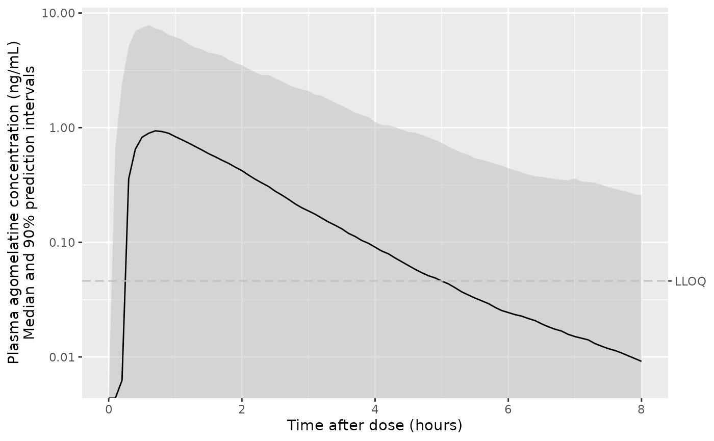
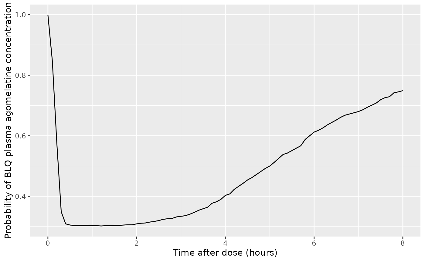
ggplot(d_plot, aes(x = time, y = prob_blq_calmt)) +
  geom_line() +
  labs(
    x = "Time after dose (hours)",
    y = "Probability of BLQ plasma agomelatine concentration"
  )
ggplot(d_plot, aes(x = time, y = Q50_c3oh, ymin = Q05_c3oh, ymax = Q95_c3oh)) +
  geom_ribbon(colour = NA, linetype = "63", fill = "gray", alpha = 0.5) +
  geom_line() +
  geom_hline(yintercept = 0.460, linetype = "63", colour = "gray") +
  scale_y_log10(sec.axis = sec_axis(transform = identity, breaks = 0.460, labels = "LLOQ")) +
  labs(
    x = "Time after dose (hours)",
    y = paste0("Plasma 3-hydroxy-agomelatine concentration (", conc_unit, ")\nMedian and 90% prediction intervals")
  )
#> Warning in scale_y_log10(sec.axis = sec_axis(transform = identity, breaks = 0.46, : log-10 transformation introduced infinite values.
#> log-10 transformation introduced infinite values.
#> log-10 transformation introduced infinite values.
#> log-10 transformation introduced infinite values.
#> log-10 transformation introduced infinite values.
#> log-10 transformation introduced infinite values.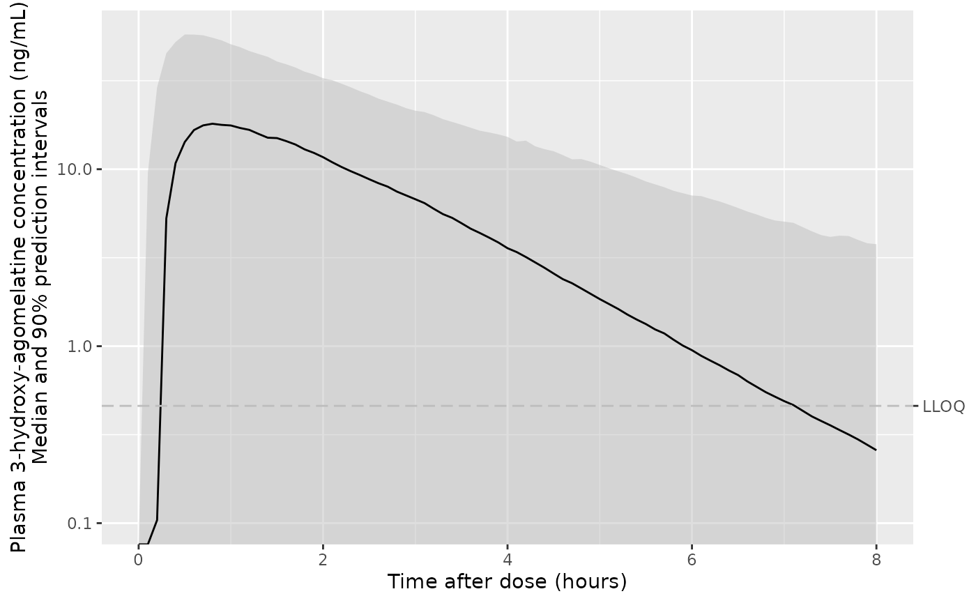
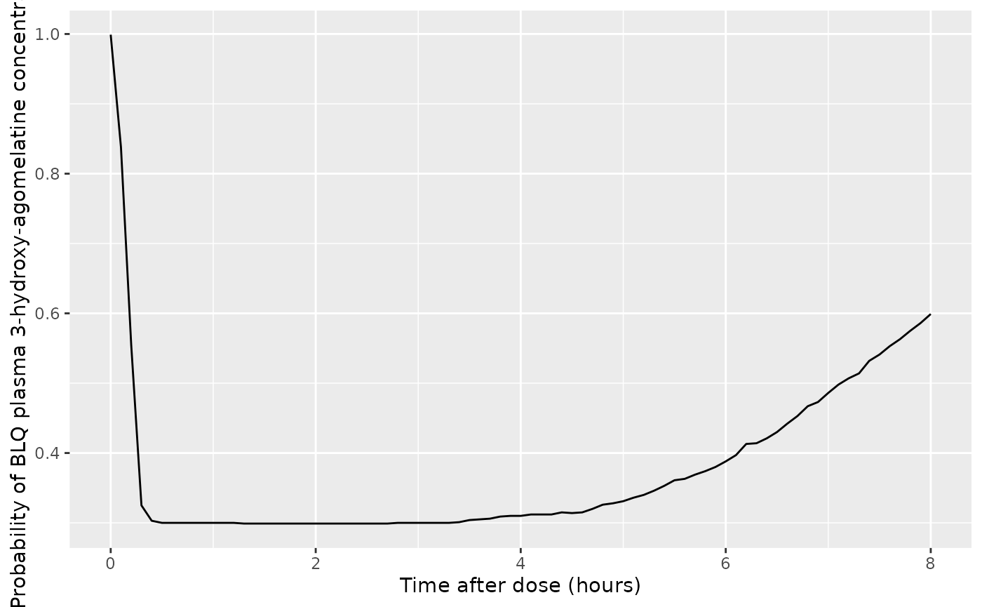
A figure for BQL 3-hydroxy-agomelatine is not in the original paper. It is added here for completeness.
ggplot(d_plot, aes(x = time, y = prob_blq_c3oh)) +
  geom_line() +
  labs(
    x = "Time after dose (hours)",
    y = "Probability of BLQ plasma 3-hydroxy-agomelatine concentration"
  )
ggplot(d_plot, aes(x = time, y = Q50_c7dm, ymin = Q05_c7dm, ymax = Q95_c7dm)) +
  geom_ribbon(colour = NA, linetype = "63", fill = "gray", alpha = 0.5) +
  geom_line() +
  geom_hline(yintercept = 0.137, linetype = "63", colour = "gray") +
  scale_y_log10(sec.axis = sec_axis(transform = identity, breaks = 0.137, labels = "LLOQ")) +
  labs(
    x = "Time after dose (hours)",
    y = paste0("Plasma 7-desmethyl-agomelatine concentration (", conc_unit, ")\nMedian and 90% prediction intervals")
  )
#> Warning in scale_y_log10(sec.axis = sec_axis(transform = identity, breaks = 0.137, : log-10 transformation introduced infinite values.
#> log-10 transformation introduced infinite values.
#> log-10 transformation introduced infinite values.
#> log-10 transformation introduced infinite values.
#> log-10 transformation introduced infinite values.
#> log-10 transformation introduced infinite values.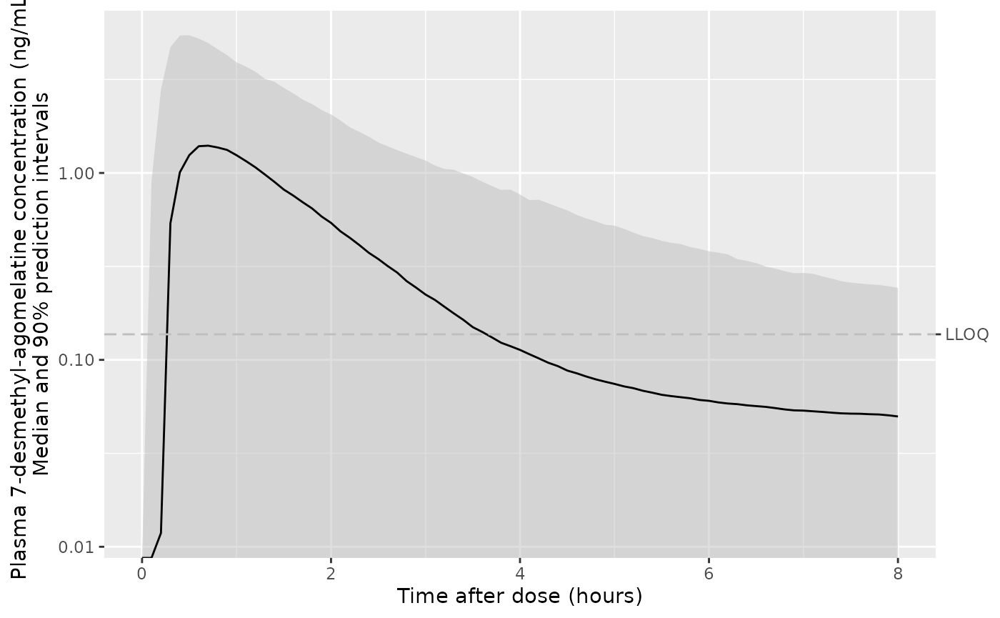
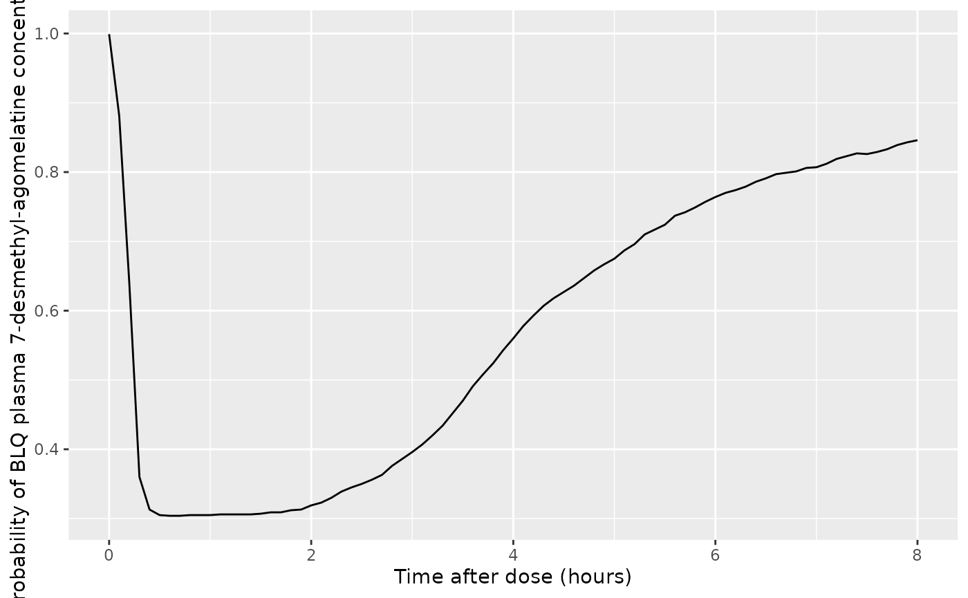
ggplot(d_plot, aes(x = time, y = prob_blq_c7dm)) +
  geom_line() +
  labs(
    x = "Time after dose (hours)",
    y = "Probability of BLQ plasma 7-desmethyl-agomelatine concentration"
  )