Omecamtiv mecarbil (Trivedi 2021)
Source:vignettes/articles/Trivedi_2021_omecamtivMecarbil.Rmd
Trivedi_2021_omecamtivMecarbil.RmdModel and source
- Citation: Trivedi A, Sohn W, Kulkarni P, Jafarinasabian P, Zhang H, Spring M, Flach S, Abbasi S, Wahlstrom J, Lee E, Dutta S. (2021). Evaluation of drug-drug interaction potential between omecamtiv mecarbil and rosuvastatin, a BCRP substrate, with a clinical study in healthy subjects and using a physiologically-based pharmacokinetic model. Clin Transl Sci 14(6):2510-2520. doi:10.1111/cts.13118.
- Description: Two-compartment oral population pharmacokinetic reduction of the Simcyp minimal-PBPK-with-single-adjusting-compartment (SAC) compound model for the cardiac myosin activator omecamtiv mecarbil in healthy adults (Trivedi 2021). Distribution was fitted by the authors as an ordinary two-compartment model to intravenous data (k12, k21 and the central volume Vc, with Vsac = Vc * k12 / k21) and then held fixed while first-order absorption ka and the apparent oral clearance CLpo were fitted to oral single- and multiple-dose data, so the Simcyp compound layer IS a two-compartment model with first-order absorption and needs no platform physiology to encode. Volumes are per kg body weight (Vss 3.8575 L/kg, Vsac 2.369 L/kg, systemic compartment Vss - Vsac); clearance is not weight-scaled. Inter- individual variability is the compound file’s 30% CV on ka, CLpo and Vss (Supplementary Table S1 workbook), with Vsac held fixed as Simcyp does, so all Vss variability falls on the systemic volume. Elimination uses the apparent oral clearance with bioavailability 1; the typical-value reduction reproduces the medians of the 50 deposited Simcyp virtual subjects (Cmax, Tmax, AUC0-48 after 50 mg) within 7.5%. The paper’s main result, rosuvastatin (BCRP substrate) exposure with omecamtiv mecarbil co-administration, runs on a Simcyp library full-PBPK/ADAM rosuvastatin compound file with transporter kinetics and is NOT reproducible from this model.
- Article: https://doi.org/10.1111/cts.13118
- Supplement (Supplementary Materials PDF and the Simcyp output workbook deposited as Supplementary Table S1): https://www.ncbi.nlm.nih.gov/pmc/articles/PMC8604240/
What this model is, and what it is not
Trivedi 2021 measured the effect of a single 50 mg oral dose of omecamtiv mecarbil (OM), an in-vitro BCRP inhibitor, on a single 10 mg oral dose of rosuvastatin in 14 healthy adults. They then built a Simcyp (V17.1) PBPK model to extrapolate the interaction to 50 mg twice-daily dosing.
The PBPK analysis has two layers, and only one of them can be encoded outside Simcyp.
-
Omecamtiv mecarbil (the perpetrator) is a two-compartment
model. The authors fitted an ordinary two-compartment model to
data after a 35 mg intravenous dose with SAAM II (
k12,k21,k10,Vc). They fixed that distribution in Simcyp’s minimal PBPK model, with a single adjusting compartment (SAC) whose volume isVsac = Vc * k12 / k21. Then they fitted a first-order absorption ratekaand an apparent oral clearanceCLpoto oral data. Every input is printed in Table 3, and the as-run values are in the Simcyp workbook deposited as Supplementary Table S1. That layer is what this package ships. -
Rosuvastatin (the victim) and the DDI are not
reproducible. Rosuvastatin runs on the Simcyp library compound
file: a full PBPK model with the ADAM gut model, a permeability-limited
liver, and OATP1B1/1B3, BCRP and MRP4 transporter kinetics
(Supplementary Table S3). The interaction acts through a BCRP
Kiof 0.05 uM in the gut, liver and kidney. Both depend on the platform’s physiology and its transporter-abundance scaling, and neither is published. The DDI ratios (Table 6 and Supplementary Table S2) are therefore not reproduced here.
Population
The omecamtiv mecarbil compound model draws on six clinical studies in healthy adults (Trivedi 2021 Table 1):
| Study | OM dose | Route | n | Women | Age (y) | Role |
|---|---|---|---|---|---|---|
| Study 5 | 35 mg single dose | IV | 7 | 0% | 21-45 | Distribution (SAAM II) |
| Study 1 | 50 mg single dose | oral | 14 | 43% | 22-54 |
ka, CLpo fit |
| Study 2 | 25 mg b.i.d., 7 days | oral | 20 | 30% | 22-45 |
ka, CLpo fit |
| Study 3 | 50 mg b.i.d., 7 days | oral | 13 | 8% | 20-35 | Verification |
| Study 4 | 25 mg b.i.d. | oral | 13 | 50% | 22-54 | Verification |
| OM-rosuvastatin DDI | 50 mg single dose | oral | 14 | 57% | 18-50 | DDI study |
The DDI-study participants (Supplementary Table S1) had a mean (SD) age of 34.1 (9.71) years and a mean weight of 70.4 (13.1) kg. They were 71.4% White, 21.4% Black and 7.1% multiple race. Table 3 converts the fitted volumes to per-kg values using a mean body weight of 83.79 kg.
readModelDb("Trivedi_2021_omecamtivMecarbil")()$population[c(
  "n_subjects",
  "n_studies",
  "sex_female_pct",
  "dose_range"
)]
#> $n_subjects
#> [1] 81
#>
#> $n_studies
#> [1] 6
#>
#> $sex_female_pct
#> [1] 34
#>
#> $dose_range
#> [1] "35 mg single intravenous dose (study 5, distribution fit); 50 mg single oral dose (study 1 and the rosuvastatin DDI study); 25 mg and 50 mg oral twice daily for 7-14 days (studies 2-4)."
Source trace
Every value is the as-run Simcyp compound-file input from the
deposited S1 workbook (sheet Input Sheet, column
Inhibitor 1, compound
AMG 423_target formulation). Each one agrees with the
rounded value in Table 3.
| Parameter / equation | Value | Source location |
|---|---|---|
lka (ka) |
0.2234 1/h | S1 workbook ka (1/h); Table 3 0.220 ‘Parameterized’;
Results 0.22 (0.18-0.26) |
lcl (CLpo, CL/F) |
10.81 L/h | S1 workbook CL (po) (L/h); Table 3 10.8
‘Parameterized’; Results 10.8 (10.3-11.3) |
lvss (Vss) |
3.8575 L/kg | S1 workbook Vss (L/kg); Table 3 3.86 L/kg (323.3 L /
83.79 kg) |
lvp (Vsac) |
2.369 L/kg | S1 workbook Volume [Vsac] (L/kg); Table 3 2.37 L/kg
(198.5 L / 83.79 kg) |
lk12 (SAC kin) |
0.31955 1/h | S1 workbook SAC kin (1/h); Table 3 / Results k12 =
0.319 (0.186-0.452) |
lk21 (SAC kout) |
0.2 1/h | S1 workbook SAC kout (1/h); Table 3 / Results k21 =
0.200 (0.136-0.265) |
etalka, etalcl, etalvss
|
log(1 + 0.3^2) = 0.0862 | S1 workbook CV ka (%), CV CL (po) (%),
CV Vss (%) = 30 |
propSd |
0 (fixed) | No residual-error model in a Simcyp simulation |
| fa = 1, no lag | n/a | S1 workbook fa = 1, lag time (h) = 0;
Methods ‘first-order kinetics’ |
vc = WT * (Vss - Vsac) |
1.4885 L/kg typical | Methods (Vss = Vc + Vsac); Table 3 Vc 1.49 L/kg |
| systemic-volume floor 0.035 L/kg | n/a | Smallest Inhibitor 1 Vsys among the 50 S1 workbook
subjects (0.0347 L/kg) |
d/dt(central), d/dt(peripheral1)
|
n/a | Methods ‘OM model development’ (two-compartment, k12 / k21) |
Cc = 1000 * central / vc |
n/a | mg / L to ng/mL (Tables 4-5 units) |
The Table 3 arithmetic closes on the paper’s own numbers:
vc_L <- 124.7
k12 <- 0.319
k21 <- 0.200
k10 <- 0.098
wt_mean <- 83.79
arith <- data.frame(
  Quantity = c(
    "Vsac = Vc * k12 / k21 (L)",
    "Vss = Vc + Vsac (L)",
    "Vc per kg (L/kg)",
    "Vsac per kg (L/kg)",
    "Vss per kg (L/kg)"
  ),
  Recomputed = c(
    vc_L * k12 / k21,
    vc_L * (1 + k12 / k21),
    vc_L / wt_mean,
    198.5 / wt_mean,
    323.3 / wt_mean
  ),
  Printed = c(198.5, 323.3, 1.49, 2.37, 3.86),
  `As run (S1 workbook)` = c(NA, NA, 3.8575 - 2.369, 2.369, 3.8575),
  check.names = FALSE
)
arith$`% diff vs printed` <- 100 * (arith$Recomputed / arith$Printed - 1)
knitr::kable(arith, digits = 4, caption = "Trivedi 2021 Table 3 and Results arithmetic.")| Quantity | Recomputed | Printed | As run (S1 workbook) | % diff vs printed |
|---|---|---|---|---|
| Vsac = Vc * k12 / k21 (L) | 198.8965 | 198.50 | NA | 0.1997 |
| Vss = Vc + Vsac (L) | 323.5965 | 323.30 | NA | 0.0917 |
| Vc per kg (L/kg) | 1.4882 | 1.49 | 1.4885 | -0.1178 |
| Vsac per kg (L/kg) | 2.3690 | 2.37 | 2.3690 | -0.0414 |
| Vss per kg (L/kg) | 3.8585 | 3.86 | 3.8575 | -0.0400 |
Model structure checks
mod <- readModelDb("Trivedi_2021_omecamtivMecarbil")
ui <- rxode2::rxode(mod)
# The model has both `cl` and `vc`; confirm rxode2 integrates the explicit
# ODEs rather than silently swapping in a linCmt() solution.
stopifnot(is.null(ui$linCmt))
mod_typ <- rxode2::zeroRe(mod)

# Typical-value terminal half-life from the micro-constants at the
# Simcyp reference body weight of 80.7 kg (S1 workbook).
wt_ref <- 80.7
kel <- 10.81 / ((3.8575 - 2.369) * wt_ref)
sum_k <- kel + 0.31955 + 0.2
beta <- (sum_k - sqrt(sum_k^2 - 4 * kel * 0.2)) / 2
cat(sprintf("Typical terminal half-life at %.1f kg: %.1f h\n", wt_ref, log(2) / beta))
#> Typical terminal half-life at 80.7 kg: 22.3 h
For a linear model, the oral AUC(0,inf) must equal
Dose / CLpo whatever the body weight or the distribution.
This is how Simcyp’s in vivo CLpo input is defined. The
check solves the typical subject with tight tolerances.
ev_id <- rxode2::et(amt = 50, cmt = "depot") |>
  rxode2::et(c(seq(0, 24, by = 0.1), seq(25, 1500, by = 1))) |>
  as.data.frame() |>
  dplyr::mutate(id = 1L, WT = wt_ref)
sim_id <- as.data.frame(rxode2::rxSolve(
  mod_typ,
  ev_id,
  rtol = 1e-10,
  atol = 1e-12,
  returnType = "data.frame"
))
#> ℹ omega/sigma items treated as zero: 'etalka', 'etalcl', 'etalvss'
conc_id <- sim_id |>
  dplyr::filter(!is.na(Cc)) |>
  dplyr::mutate(id = 1L, Cc = pmax(Cc, 0))
nca_id <- PKNCA::pk.nca(PKNCA::PKNCAdata(
  PKNCA::PKNCAconc(conc_id, Cc ~ time | id),
  PKNCA::PKNCAdose(data.frame(id = 1L, time = 0, amt = 50), amt ~ time | id),
  intervals = data.frame(start = 0, end = Inf, aucinf.obs = TRUE, cmax = TRUE)
))
auc_inf <- as.data.frame(nca_id) |>
  dplyr::filter(PPTESTCD == "aucinf.obs") |>
  dplyr::pull(PPORRES)
auc_expected <- 50 * 1000 / 10.81
cat(sprintf(
  "AUC(0,inf) = %.1f ng*h/mL; Dose / CLpo = %.1f ng*h/mL (%.3f%% apart)\n",
  auc_inf,
  auc_expected,
  100 * (auc_inf / auc_expected - 1)
))
#> AUC(0,inf) = 4625.3 ng*h/mL; Dose / CLpo = 4625.3 ng*h/mL (-0.002% apart)
# Trapezoidal error on a 0.1 h / 1 h grid is ~0.01%; 0.5% is 50x headroom.
stopifnot(abs(auc_inf / auc_expected - 1) < 0.005)
Known-answer check against the deposited Simcyp run
The S1 workbook is the Simcyp output of the OM-rosuvastatin DDI
simulation. It holds 5 trials of 10 subjects, 18-65 years, with 50%
women in the input sheet. Omecamtiv mecarbil is the inhibitor, given as
a single 50 mg oral dose. The workbook reports each virtual subject’s
omecamtiv mecarbil Cmax, Tmax and AUC(0-48) (sheet
AUC0(Inh 1)(CPlasma)), and the population mean, 5th and
95th percentile profile (sheet
Conc Profiles CSys(CPlasma)). The values below were
transcribed from those sheets.
deposit_median <- c(Cmax = 127.702, Tmax = 4.5251, AUC48 = 3619.68)
deposit_profile <- tibble::tribble(
  ~time, ~mean, ~p5, ~p95,
  0.0000, 0.000, 0.00000, 0.000,
  0.4800, 91.356, 15.89200, 373.430,
  0.9600, 136.710, 28.14900, 518.310,
  1.9200, 170.090, 43.78500, 565.660,
  2.8800, 174.910, 51.96600, 533.690,
  4.0801, 167.660, 59.04000, 421.700,
  6.0001, 148.590, 64.34000, 307.720,
  7.9201, 130.530, 64.46600, 240.230,
  12.0001, 102.550, 51.27300, 168.050,
  16.0801, 84.369, 40.95600, 135.160,
  23.7601, 62.650, 21.52800, 95.306,
  36.0001, 42.454, 3.86910, 71.183,
  48.0000, 30.400, 0.65996, 57.636
)
The typical subject at the Simcyp reference weight should sit at the centre of the deposited distribution. It has no inter-individual variability, and the reduction uses bioavailability 1:
ev_48 <- rxode2::et(amt = 50, cmt = "depot") |>
  rxode2::et(seq(0, 48, by = 0.05)) |>
  as.data.frame() |>
  dplyr::mutate(id = 1L, WT = wt_ref)
sim_48 <- as.data.frame(rxode2::rxSolve(mod_typ, ev_48, returnType = "data.frame")) |>
  dplyr::mutate(id = 1L)
#> ℹ omega/sigma items treated as zero: 'etalka', 'etalcl', 'etalvss'
nca_48 <- PKNCA::pk.nca(PKNCA::PKNCAdata(
  PKNCA::PKNCAconc(sim_48, Cc ~ time | id),
  PKNCA::PKNCAdose(data.frame(id = 1L, time = 0, amt = 50), amt ~ time | id),
  intervals = data.frame(start = 0, end = 48, cmax = TRUE, tmax = TRUE, auclast = TRUE)
))
typ_48 <- as.data.frame(nca_48) |>
  dplyr::select(PPTESTCD, PPORRES) |>
  tidyr::pivot_wider(names_from = PPTESTCD, values_from = PPORRES)
typ_cmp <- data.frame(
  Metric = c("Cmax (ng/mL)", "Tmax (h)", "AUC0-48 (ng*h/mL)"),
  `Typical reduction` = c(typ_48$cmax, typ_48$tmax, typ_48$auclast),
  `Deposited median (50 subjects)` = unname(deposit_median),
  check.names = FALSE
)
typ_cmp$`% diff` <- 100 * (typ_cmp$`Typical reduction` / typ_cmp$`Deposited median (50 subjects)` - 1)
knitr::kable(typ_cmp, digits = 2, caption = "Typical subject vs the deposited Simcyp virtual subjects.")| Metric | Typical reduction | Deposited median (50 subjects) | % diff |
|---|---|---|---|
| Cmax (ng/mL) | 128.16 | 127.70 | 0.35 |
| Tmax (h) | 4.85 | 4.53 | 7.18 |
| AUC0-48 (ng*h/mL) | 3548.35 | 3619.68 | -1.97 |
# Measured: Cmax +0.4%, Tmax +7.2%, AUC0-48 -2.0%. A dose, clearance or
# volume transcription error moves these by tens of percent.
stopifnot(all(abs(typ_cmp$`% diff`) < 10))
Next, a stochastic cohort of the same design (200 subjects, 50 mg single dose). Body weight is drawn as normal with mean 80.7 kg (the Simcyp reference weight) and SD 13 kg (the DDI study’s SD), redrawn outside 50-120 kg. The robust summaries are compared with the deposited subjects:
set.seed(8604240)
rxode2::rxSetSeed(8604240)

draw_wt <- function(n, mean = 80.7, sd = 13, lo = 50, hi = 120) {
  wt <- numeric(0)
  while (length(wt) < n) {
    x <- stats::rnorm(n, mean, sd)
    wt <- c(wt, x[x >= lo & x <= hi])
  }
  wt[seq_len(n)]
}

n_dep <- 200L
ev_dep <- rxode2::et(amt = 50, cmt = "depot") |>
  rxode2::et(c(0, seq(0.24, 48, by = 0.24))) |>
  rxode2::et(id = seq_len(n_dep)) |>
  as.data.frame() |>
  dplyr::left_join(data.frame(id = seq_len(n_dep), WT = draw_wt(n_dep)), by = "id")
sim_dep <- as.data.frame(rxode2::rxSolve(mod, ev_dep, returnType = "data.frame"))

nca_dep <- PKNCA::pk.nca(PKNCA::PKNCAdata(
  PKNCA::PKNCAconc(dplyr::filter(sim_dep, !is.na(Cc)), Cc ~ time | id),
  PKNCA::PKNCAdose(data.frame(id = seq_len(n_dep), time = 0, amt = 50), amt ~ time | id),
  intervals = data.frame(start = 0, end = 48, cmax = TRUE, tmax = TRUE, auclast = TRUE)
))
coh <- as.data.frame(nca_dep) |>
  dplyr::group_by(PPTESTCD) |>
  dplyr::summarise(median = stats::median(PPORRES), .groups = "drop") |>
  tidyr::pivot_wider(names_from = PPTESTCD, values_from = median)
coh_cmp <- data.frame(
  Metric = c("Median Cmax (ng/mL)", "Median Tmax (h)", "Median AUC0-48 (ng*h/mL)"),
  `Simulated cohort` = c(coh$cmax, coh$tmax, coh$auclast),
  `Deposited Simcyp subjects` = unname(deposit_median),
  check.names = FALSE
)
coh_cmp$`% diff` <- 100 * (coh_cmp$`Simulated cohort` / coh_cmp$`Deposited Simcyp subjects` - 1)
knitr::kable(coh_cmp, digits = 2, caption = "Cohort medians vs the deposited Simcyp virtual subjects.")| Metric | Simulated cohort | Deposited Simcyp subjects | % diff |
|---|---|---|---|
| Median Cmax (ng/mL) | 123.69 | 127.70 | -3.14 |
| Median Tmax (h) | 4.32 | 4.53 | -4.53 |
| Median AUC0-48 (ng*h/mL) | 3295.79 | 3619.68 | -8.95 |
# Medians are robust to which subjects land in the tails; measured
# differences are within about 10% across seeds (AUC0-48 runs 7-9% low).
stopifnot(all(abs(coh_cmp$`% diff`) < 20))
coh_prof <- sim_dep |>
  dplyr::filter(!is.na(Cc)) |>
  dplyr::group_by(time) |>
  dplyr::summarise(
    mean = mean(Cc),
    p5 = stats::quantile(Cc, 0.05),
    p95 = stats::quantile(Cc, 0.95),
    .groups = "drop"
  )
ggplot() +
  geom_ribbon(data = coh_prof, aes(time, ymin = p5, ymax = p95), fill = "steelblue", alpha = 0.25) +
  geom_line(data = coh_prof, aes(time, mean), colour = "steelblue", linewidth = 1) +
  geom_point(data = deposit_profile, aes(time, mean), colour = "black") +
  geom_errorbar(data = deposit_profile, aes(time, ymin = p5, ymax = p95), colour = "black", width = 0.6) +
  labs(
    x = "Time after 50 mg oral dose (h)",
    y = "Omecamtiv mecarbil plasma concentration (ng/mL)",
    caption = paste(
      "Blue: this model, 200 virtual subjects (mean and 5th-95th percentile).",
      "Black: deposited Simcyp run, 50 subjects (S1 workbook).",
      sep = "\n"
    )
  ) +
  theme_bw()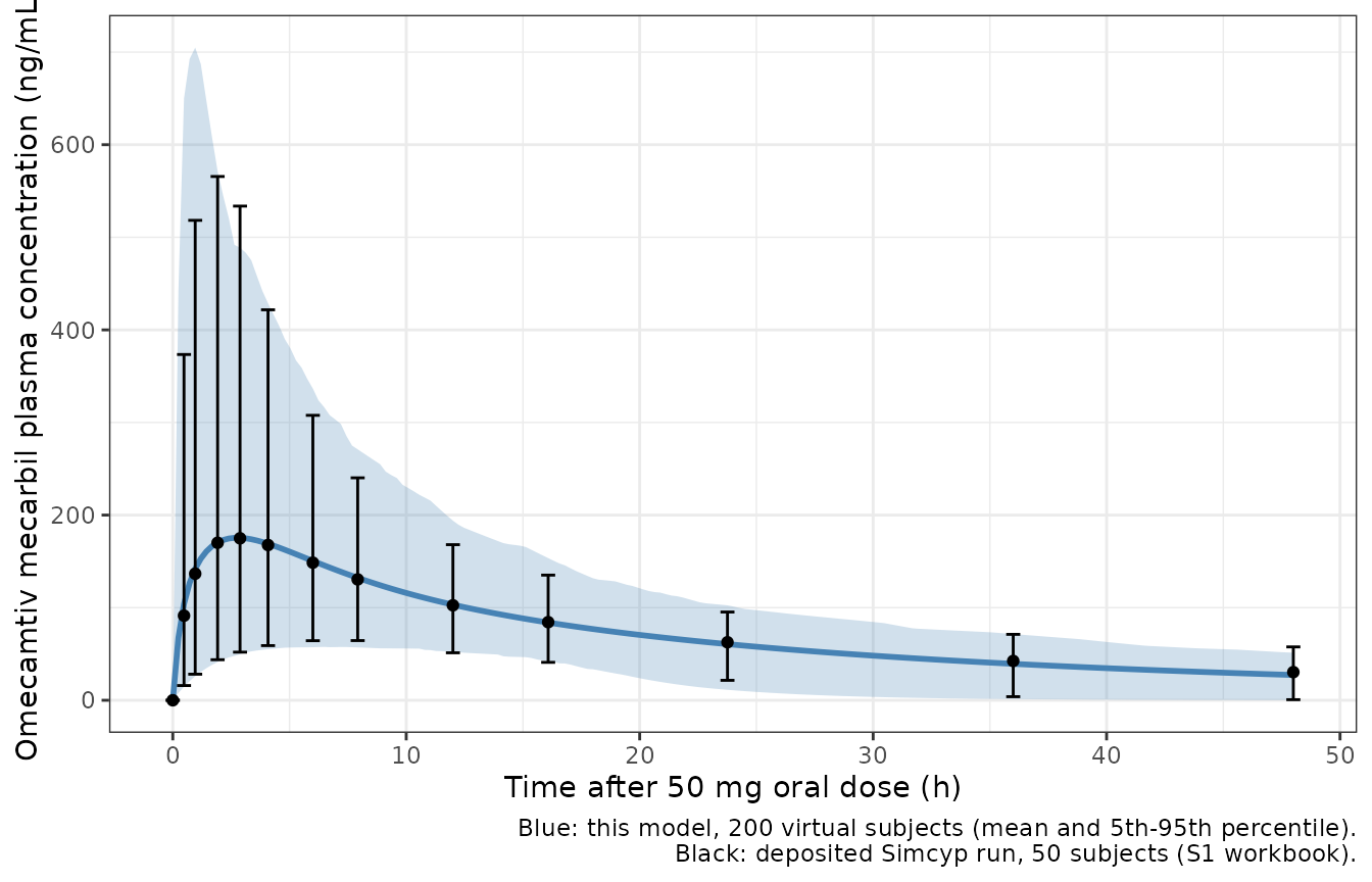
The deposited mean profile peaks near 2.9 h, well before the median individual Tmax of 4.5 h. This comes from subjects whose systemic volume is very small. When a subject’s sampled Vss falls close to the fixed Vsac, their systemic compartment shrinks and they get a tall, early spike. The reduction reproduces this because it applies the variability to Vss and not to Vc (see Assumptions and deviations).
Replicating Tables 4 and 5 (Simcyp-simulated omecamtiv mecarbil exposure)
Tables 4 and 5 compare the Simcyp-simulated exposures of the four
oral studies with the observed values. Each virtual study is simulated
here with the design of Table 1: 10 trials of the study’s size (130-200
subjects), a single dose or twice-daily dosing, and a final morning dose
on the reported day. Table 4 footnotes define the intervals:
AUC(0-144) after the single dose, and
AUC(0-12) on day 1 and day 8. Table 5 reports study 4 on
day 15.
make_study <- function(label, dose, n, n_doses, id_offset) {
  dose_times <- (seq_len(n_doses) - 1) * 12
  last <- max(dose_times)
  obs <- sort(unique(c(
    seq(0, 12, by = 0.1),
    seq(last, last + 12, by = 0.1),
    if (n_doses == 1) seq(12, 144, by = 0.5) else seq(0, last, by = 1)
  )))
  ids <- id_offset + seq_len(n)
  dose_rows <- expand.grid(id = ids, time = dose_times) |>
    dplyr::mutate(evid = 1L, amt = dose, cmt = "depot")
  obs_rows <- expand.grid(id = ids, time = obs) |>
    dplyr::mutate(evid = 0L, amt = 0, cmt = "central")
  dplyr::bind_rows(dose_rows, obs_rows) |>
    dplyr::left_join(data.frame(id = ids, WT = draw_wt(n)), by = "id") |>
    dplyr::mutate(study = label, last_dose = last) |>
    dplyr::arrange(id, time, dplyr::desc(evid))
}

events <- dplyr::bind_rows(
  make_study("Study 1: 50 mg single dose", 50, 140L, 1L, 0L),
  make_study("Study 2: 25 mg b.i.d., day 8", 25, 200L, 15L, 1000L),
  make_study("Study 3: 50 mg b.i.d., day 8", 50, 130L, 15L, 2000L),
  make_study("Study 4: 25 mg b.i.d., day 15", 25, 130L, 29L, 3000L)
)
stopifnot(!anyDuplicated(events[, c("id", "time", "evid")]))

sim <- as.data.frame(rxode2::rxSolve(
  mod,
  events,
  keep = c("study", "last_dose"),
  returnType = "data.frame"
))
sim |>
  dplyr::filter(!is.na(Cc)) |>
  dplyr::mutate(tad_last = time - last_dose) |>
  dplyr::filter(tad_last >= 0, tad_last <= 12 | grepl("single", study)) |>
  dplyr::group_by(study, tad_last) |>
  dplyr::summarise(
    median = stats::median(Cc),
    p5 = stats::quantile(Cc, 0.05),
    p95 = stats::quantile(Cc, 0.95),
    .groups = "drop"
  ) |>
  dplyr::filter(tad_last <= 48) |>
  ggplot(aes(tad_last, median)) +
  geom_ribbon(aes(ymin = p5, ymax = p95), alpha = 0.25) +
  geom_line() +
  facet_wrap(~study, scales = "free") +
  labs(
    x = "Time after the (last) dose (h)",
    y = "Omecamtiv mecarbil (ng/mL)",
    caption = "Median and 5th-95th percentile. Compare with Figures S3 and S4 of Trivedi 2021."
  ) +
  theme_bw()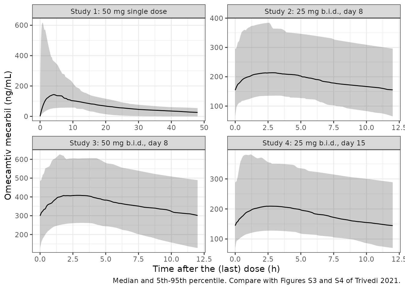
PKNCA validation
conc <- sim |>
  dplyr::filter(!is.na(Cc)) |>
  dplyr::mutate(Cc = pmax(Cc, 0)) |>
  dplyr::select(id, time, Cc, study, last_dose)
dose <- events |>
  dplyr::filter(evid == 1L) |>
  dplyr::select(id, time, amt, study)

intervals <- dplyr::bind_rows(
  data.frame(
    study = "Study 1: 50 mg single dose",
    start = c(0, 0),
    end = c(144, Inf),
    cmax = c(TRUE, FALSE),
    tmax = c(TRUE, FALSE),
    auclast = c(TRUE, FALSE),
    aucinf.obs = c(FALSE, TRUE)
  ),
  data.frame(
    study = c("Study 2: 25 mg b.i.d., day 8", "Study 3: 50 mg b.i.d., day 8"),
    start = 0,
    end = 12,
    cmax = TRUE,
    tmax = TRUE,
    auclast = TRUE,
    aucinf.obs = FALSE
  ),
  data.frame(
    study = c(
      "Study 2: 25 mg b.i.d., day 8",
      "Study 3: 50 mg b.i.d., day 8",
      "Study 4: 25 mg b.i.d., day 15"
    ),
    start = c(168, 168, 336),
    end = c(180, 180, 348),
    cmax = TRUE,
    tmax = TRUE,
    auclast = TRUE,
    aucinf.obs = FALSE
  )
)

nca <- PKNCA::pk.nca(PKNCA::PKNCAdata(
  PKNCA::PKNCAconc(conc, Cc ~ time | study + id, concu = "ng/mL", timeu = "h"),
  PKNCA::PKNCAdose(dose, amt ~ time | study + id, doseu = "mg"),
  intervals = intervals
))
nca_df <- as.data.frame(nca) |>
  dplyr::mutate(
    arm = dplyr::case_when(
      start == 0 & grepl("b.i.d.", study) ~ paste(sub(", day.*", "", study), "day 1"),
      TRUE ~ study
    )
  )
Table 4 and Table 5 report the Simcyp-simulated Cmax and AUC as arithmetic means and Tmax as a median. The simulated cohort is summarised the same way before comparison. The day-8 and day-15 pre-dose concentrations are read directly from the simulation at the time of the final dose.
sim_summary <- nca_df |>
  dplyr::filter(PPTESTCD %in% c("cmax", "tmax", "auclast", "aucinf.obs")) |>
  dplyr::group_by(arm, PPTESTCD) |>
  dplyr::summarise(
    PPORRES = if (PPTESTCD[1] == "tmax") stats::median(PPORRES) else mean(PPORRES),
    .groups = "drop"
  )
ctrough <- sim |>
  dplyr::filter(!is.na(Cc), grepl("b.i.d.", study), time == last_dose) |>
  dplyr::group_by(arm = study) |>
  dplyr::summarise(PPORRES = mean(Cc), .groups = "drop") |>
  dplyr::mutate(PPTESTCD = "ctrough")
sim_summary <- dplyr::bind_rows(sim_summary, ctrough)

# Trivedi 2021 Table 4 (studies 1-2) and Table 5 (studies 3-4), 'Simulated'
# rows. auclast is AUC(0-144) for study 1 and AUC(0-12) otherwise; study 4
# 'AUCtau' is AUC(0-12) on day 15.
published <- tibble::tribble(
  ~arm, ~cmax, ~tmax, ~auclast, ~aucinf.obs, ~ctrough,
  "Study 1: 50 mg single dose", 218, 4.6, 4956, 5227, NA,
  "Study 2: 25 mg b.i.d. day 1", 114, 4.6, 930, NA, NA,
  "Study 2: 25 mg b.i.d., day 8", 256, 3.1, 2512, NA, 162,
  "Study 3: 50 mg b.i.d. day 1", 216, 4.6, 1768, NA, NA,
  "Study 3: 50 mg b.i.d., day 8", 506, 3.1, 5026, NA, 326,
  "Study 4: 25 mg b.i.d., day 15", 266, 3.1, 2624, NA, NA
)

cmp <- nlmixr2lib::ncaComparisonTable(
  simulated = sim_summary,
  reference = published,
  by = "arm",
  units = c(
    cmax = "ng/mL",
    tmax = "h",
    auclast = "ng*h/mL",
    aucinf.obs = "ng*h/mL",
    ctrough = "ng/mL"
  ),
  tolerance_pct = 20
)
knitr::kable(
  cmp,
  caption = paste(
    "This model vs the Simcyp-simulated values of Trivedi 2021 Tables 4-5",
    "(Cmax, AUC and pre-dose concentration as means; Tmax as medians)."
  )
)| NCA parameter | arm | Reference | Simulated | % diff |
|---|---|---|---|---|
| Cmax (ng/mL) | Study 1: 50 mg single dose | 218 | 207 | -4.9% |
| Cmax (ng/mL) | Study 2: 25 mg b.i.d. day 1 | 114 | 91.6 | -19.6% |
| Cmax (ng/mL) | Study 2: 25 mg b.i.d., day 8 | 256 | 237 | -7.3% |
| Cmax (ng/mL) | Study 3: 50 mg b.i.d. day 1 | 216 | 154 | -28.7%* |
| Cmax (ng/mL) | Study 3: 50 mg b.i.d., day 8 | 506 | 424 | -16.2% |
| Cmax (ng/mL) | Study 4: 25 mg b.i.d., day 15 | 266 | 229 | -14.0% |
| Tmax (h) | Study 1: 50 mg single dose | 4.6 | 4.3 | -6.5% |
| Tmax (h) | Study 2: 25 mg b.i.d. day 1 | 4.6 | 4.8 | +4.3% |
| Tmax (h) | Study 2: 25 mg b.i.d., day 8 | 3.1 | 3.1 | -0.0% |
| Tmax (h) | Study 3: 50 mg b.i.d. day 1 | 4.6 | 4.5 | -2.2% |
| Tmax (h) | Study 3: 50 mg b.i.d., day 8 | 3.1 | 3.1 | -0.0% |
| Tmax (h) | Study 4: 25 mg b.i.d., day 15 | 3.1 | 3.1 | +0.0% |
| AUC0-∞ (obs) (ng*h/mL) | Study 1: 50 mg single dose | 5230 | 4740 | -9.3% |
| AUClast (ng*h/mL) | Study 1: 50 mg single dose | 4960 | 4510 | -8.9% |
| AUClast (ng*h/mL) | Study 2: 25 mg b.i.d. day 1 | 930 | 767 | -17.6% |
| AUClast (ng*h/mL) | Study 2: 25 mg b.i.d., day 8 | 2510 | 2400 | -4.3% |
| AUClast (ng*h/mL) | Study 3: 50 mg b.i.d. day 1 | 1770 | 1390 | -21.2%* |
| AUClast (ng*h/mL) | Study 3: 50 mg b.i.d., day 8 | 5030 | 4420 | -12.0% |
| AUClast (ng*h/mL) | Study 4: 25 mg b.i.d., day 15 | 2620 | 2320 | -11.8% |
| Ctrough (ng/mL) | Study 2: 25 mg b.i.d., day 8 | 162 | 163 | +0.3% |
| Ctrough (ng/mL) | Study 3: 50 mg b.i.d., day 8 | 326 | 302 | -7.3% |
| Ctrough (ng/mL) | Study 4: 25 mg b.i.d., day 15 | — | 156 | — |
The AUC means depend almost entirely on CLpo and its
variability. They run 4-12% below the Simcyp means after the single dose
and at steady state, and 18-21% below for the day-1
AUC(0-12). The direction is consistent with the platform
adding clearance variability through its population physiology: the mean
of Dose / CL rises with the spread of CL. This
reduction carries only the compound file’s 30% CV. As a check,
Dose / CLpo for 50 mg is 4625 ngh/mL, and Simcyp’s mean
study-1 AUC(0,inf) of 5227 ngh/mL is 13% above it. A
log-normal 30% CV alone raises the mean by only 4.4%.
The Cmax means are driven by the right tail, the few subjects with a very small systemic volume. That makes them sensitive to the platform’s handling of those draws and to which subjects are sampled. They run 5-29% low, are shown for comparison, and are not gated.
pct <- function(arm, code) {
  s <- sim_summary$PPORRES[sim_summary$arm == arm & sim_summary$PPTESTCD == code]
  r <- published[[code]][published$arm == arm]
  100 * (s / r - 1)
}
auc_diff <- c(
  pct("Study 1: 50 mg single dose", "auclast"),
  pct("Study 1: 50 mg single dose", "aucinf.obs"),
  pct("Study 2: 25 mg b.i.d., day 8", "auclast"),
  pct("Study 3: 50 mg b.i.d., day 8", "auclast"),
  pct("Study 4: 25 mg b.i.d., day 15", "auclast")
)
print(round(auc_diff, 1))
#> [1]  -8.9  -9.3  -4.3 -12.0 -11.8
# Structural: a mis-transcribed clearance or dose moves every mean AUC by
# tens of percent. Measured median about -9% (range -4% to -12%); the bounds
# leave room for the cohort draw, per the robust-quantile rule.
stopifnot(
  abs(stats::median(auc_diff)) < 15,
  all(abs(auc_diff) < 25)
)
The observed clinical values (Tables 4-5, ‘Observed’ rows) are shown for context. The authors’ acceptance criterion was simulated within two-fold of observed. The largest misses in the paper itself are the study-1 Tmax (simulated 4.6 h vs observed 9.0 h) and the study-1 Cmax (218 vs 112 ng/mL).
observed <- tibble::tribble(
  ~Arm, ~`Cmax (ng/mL)`, ~`Tmax (h)`, ~`AUC (ng*h/mL)`,
  "Study 1: 50 mg single dose (AUC0-144)", "112 +/- 19.1", "9.0 (3.0-12.0)", "4430 +/- 1040",
  "Study 2: 25 mg b.i.d. day 1 (AUC0-12)", "77.4 +/- 21.6", "4.0 (0.5-8.0)", "687 +/- 210",
  "Study 2: 25 mg b.i.d. day 8 (AUC0-12)", "256 +/- 71.2", "2.0 (0.5-4.0)", "2570 +/- 739",
  "Study 3: 50 mg b.i.d. day 1 (AUC0-12)", "154 +/- 22", "3.0 (0.5-6.0)", "1330 +/- 217",
  "Study 3: 50 mg b.i.d. day 8 (AUC0-12)", "537 +/- 91.7", "3.0 (0.5-4.0)", "5490 +/- 1000",
  "Study 4: 25 mg b.i.d. day 15 (AUCtau)", "229 +/- 15", "2.0 (1.0-11.8)", "2520 +/- 15"
)
knitr::kable(observed, caption = "Observed omecamtiv mecarbil exposure, Trivedi 2021 Tables 4-5.")| Arm | Cmax (ng/mL) | Tmax (h) | AUC (ng*h/mL) |
|---|---|---|---|
| Study 1: 50 mg single dose (AUC0-144) | 112 +/- 19.1 | 9.0 (3.0-12.0) | 4430 +/- 1040 |
| Study 2: 25 mg b.i.d. day 1 (AUC0-12) | 77.4 +/- 21.6 | 4.0 (0.5-8.0) | 687 +/- 210 |
| Study 2: 25 mg b.i.d. day 8 (AUC0-12) | 256 +/- 71.2 | 2.0 (0.5-4.0) | 2570 +/- 739 |
| Study 3: 50 mg b.i.d. day 1 (AUC0-12) | 154 +/- 22 | 3.0 (0.5-6.0) | 1330 +/- 217 |
| Study 3: 50 mg b.i.d. day 8 (AUC0-12) | 537 +/- 91.7 | 3.0 (0.5-4.0) | 5490 +/- 1000 |
| Study 4: 25 mg b.i.d. day 15 (AUCtau) | 229 +/- 15 | 2.0 (1.0-11.8) | 2520 +/- 15 |
Assumptions and deviations
- Only the omecamtiv mecarbil layer is encoded. The rosuvastatin PBPK model and the BCRP-mediated interaction (Tables 2 and 6, Supplementary Tables S2-S4) need the Simcyp full-PBPK/ADAM rosuvastatin compound file and the platform’s transporter-abundance scaling. Neither is published, so the rosuvastatin AUC and Cmax ratios cannot be reproduced. The compound file also lists CYP2C8 and CYP3A4 inhibition, CYP3A4 induction, and OATP1B1/1B3, BCRP and MRP4 inhibition constants for omecamtiv mecarbil. Those act only on a co-simulated substrate and are not part of this model.
-
Bioavailability 1 with the apparent oral clearance.
Simcyp’s in vivo
CLpoinput fixes the oralAUC(0,inf)atDose / CLpo(fa = 1, no gut metabolism). The platform still routes the absorbed dose through a liver compartment. That applies an internal hepatic first-pass fraction computed from its own hepatic blood flow, which is not printed. Here the absorbed dose enters the systemic compartment directly, and elimination usesCLpo. The typical subject still matches the deposited Simcyp medians within 7.5% (Cmax, Tmax andAUC(0-48)). -
The SAAM II intravenous clearance is not carried.
The IV fit gave
k10 = 0.098 1/h, i.e.CL = k10 * Vc = 12.2 L/h. That is above the oralCLpo = 10.8 L/h, so taken literally it implies a bioavailability of 1.13. The final Simcyp model uses onlyCLpofor elimination (Table 3 has nok10row), and this model follows it. It is therefore an oral model. It is not a validated description of the 35 mg intravenous data. -
Variability. The 30% CVs on
ka,CLpoandVssare Simcyp’s compound-file inputs, encoded log-normally. They are not population estimates. Simcyp’s population file adds more variability through its physiology (hepatic blood flow, liver volume), which is not reproduced. As in Simcyp,Vsaccarries no variability, so all theVssvariability falls on the systemic volume. That gives the systemic volume a CV of about 70% here (log-normal Vss). The deposited run’s 50 subjects show a CV of 59% (Inhibitor 1 Vsyscv 0.59). The deposited Vss is also less skewed (skewness 0.15) than a log-normal 30% CV would give. The platform’s sampling distribution for Vss is not stated, so the log-normal form is an assumption. -
Systemic-volume floor. About 5% of
Vssdraws fall belowVsac. For those subjects the platform keeps a small positive systemic volume and shortens the SAC instead. The rule is not published. The model uses a floor of 0.035 L/kg, the smallest systemic volume among the 50 deposited subjects. The floor never acts at the typical value. -
Liver lumped into the systemic compartment.
Simcyp’s systemic volume excludes the liver, about 0.02 L/kg in the
deposited run. The workbook’s SAC clearances (
CLin37.86 L/h,CLout38.24 L/h) are consistent with that. The paper’s own Table 3 valueVc = Vss - Vsac = 1.49 L/kgis used instead. It differs by about 1.4%. - Virtual cohorts. Body weight is drawn as normal with mean 80.7 kg (the Sim-Healthy Volunteers reference weight in the S1 workbook) and SD 13 kg (the DDI study), redrawn outside 50-120 kg. Age and sex have no effect in this reduction, so they are not simulated.
- Study numbering in the supplement. The Supplementary Materials section ‘Development of the OM compound file’ calls the single 50 mg dose study ‘Study 4’ and the 25 mg b.i.d. study ‘Study 1’. The main text (Table 1, Table 4) uses ‘Study 1’ and ‘Study 2’ for the same studies. The main-text numbering is used here.
-
Study 4 observed AUC SD. Table 5 prints the
observed study 4
AUCtauas 2520 +/- 15 ng*h/mL and Cmax as 229 +/- 15 ng/mL. An SD of 15 on an AUC of 2520 is implausibly small next to every other row. It is reproduced as printed.