Omalizumab reduced TMDD design model (Brekkan 2018) • nlmixr2lib

library(nlmixr2lib)
library(rxode2)
#> rxode2 5.1.8 using 2 threads (see ?getRxThreads)
#>   no cache: create with `rxCreateCache()`
library(dplyr)
#> 
#> Attaching package: 'dplyr'
#> The following objects are masked from 'package:stats':
#> 
#>     filter, lag
#> The following objects are masked from 'package:base':
#> 
#>     intersect, setdiff, setequal, union
library(tidyr)
library(ggplot2)
library(PKNCA)
#> 
#> Attaching package: 'PKNCA'
#> The following object is masked from 'package:stats':
#> 
#>     filter

The reduced omalizumab TMDD model

Brekkan et al. (2018) asked how far a rich monoclonal-antibody trial can be cut down – fewer samples, shorter follow-up, fewer dose groups, fewer analytes – before the information it carries degrades unacceptably. To answer it they needed a reference model that could be simulated and optimized cheaply, so they took the published omalizumab / IgE quasi-equilibrium target-mediated drug disposition (TMDD) model of Hayashi et al. (2007) and reduced it: the body-weight and baseline-IgE covariate relationships were dropped, and so was the correlation between random effects.

That reduction is the model extracted here, and it is genuinely a different model from its parent rather than a restatement of it. Removing the baseline-IgE covariate removes the only thing that set the pretreatment total-IgE state, so the IgE compartment instead begins at the steady state of its own zero-order synthesis and first-order loss (ksyn * v_ige / cl_ige). That is what produces the single population baseline of 422.82 ng/mL free IgE that the paper quotes, and it is reproduced exactly below.

Three serum entities are tracked – free omalizumab, free IgE, and the omalizumab-IgE complex – coupled by instantaneous-equilibrium binding with a dissociation constant that depends on the ratio of total omalizumab to total IgE. Absorption from the subcutaneous site is first-order. Three quantities are observed: total omalizumab, total IgE, and free IgE.

Citation: Brekkan A, Jonsson S, Karlsson MO, Hooker AC. Reduced and optimized trial designs for drugs described by a target mediated drug disposition model. J Pharmacokinet Pharmacodyn. 2018;45(4):637-647. doi:10.1007/s10928-018-9594-9 (PMCID PMC6061097). Model structure and parameter values are given in Supplementary material Appendix 1 (Electronic Supplementary Material 10928_2018_9594_MOESM1_ESM.docx), Table 1A. The parent model, from which the covariate relationships and random-effect correlations were removed, is Hayashi N, Tsukamoto Y, Sallas WM, Lowe PJ. Br J Clin Pharmacol. 2007;63(5):548-561; see modellib(‘Hayashi_2007_omalizumab’).
Article: https://doi.org/10.1007/s10928-018-9594-9
PMCID: PMC6061097
Parent model: modellib("Hayashi_2007_omalizumab")

mod <- readModelDb("Brekkan_2018_omalizumab")
ui <- rxode2::rxode(mod)
#> ℹ parameter labels from comments will be replaced by 'label()'
ui
#>  ── rxode2-based free-form 3-cmt ODE model ────────────────────────────────────── 
#>  ── Initalization: ──  
#> Fixed Effects ($theta): 
#>             lka             lcl             lvc         lcl_ige          lv_ige 
#>     -0.73396918     -1.73909112      1.77495235      0.53297843      1.77495235 
#>     lcl_complex     lvc_complex           lksyn            lkd0           alpha 
#>     -1.96155185      1.28923265      1.33289358      0.06765865      0.15700000 
#>          propSd propSd_totalIgE  propSd_freeIgE 
#>      0.17000000      0.21000000      0.22000000 
#> 
#> Omega ($omega): 
#>                 etalka    etalcl    etalvc etalcl_ige  etalksyn etalcl_complex
#> etalka         0.14842 0.0000000 0.0000000  0.0000000 0.0000000      0.0000000
#> etalcl         0.00000 0.0392207 0.0000000  0.0000000 0.0000000      0.0000000
#> etalvc         0.00000 0.0000000 0.0167588  0.0000000 0.0000000      0.0000000
#> etalcl_ige     0.00000 0.0000000 0.0000000  0.0606246 0.0000000      0.0000000
#> etalksyn       0.00000 0.0000000 0.0000000  0.0000000 0.0515483      0.0000000
#> etalcl_complex 0.00000 0.0000000 0.0000000  0.0000000 0.0000000      0.1155583
#> etalvc_complex 0.00000 0.0000000 0.0000000  0.0000000 0.0000000      0.0000000
#>                etalvc_complex
#> etalka              0.0000000
#> etalcl              0.0000000
#> etalvc              0.0000000
#> etalcl_ige          0.0000000
#> etalksyn            0.0000000
#> etalcl_complex      0.0000000
#> etalvc_complex      0.0606246
#> attr(,"lotriLabels")
#> [1] "Supplement Table 1A, 'omega Ka' CV 0.40"    
#> [2] "Supplement Table 1A, 'omega CLOMA' CV 0.20" 
#> [3] "Supplement Table 1A, 'omega VOMA' CV 0.13"  
#> [4] "Supplement Table 1A, 'omega CLIGE' CV 0.25" 
#> [5] "Supplement Table 1A, 'omega ksyn' CV 0.23"  
#> [6] "Supplement Table 1A, 'omega CLcomp' CV 0.35"
#> [7] "Supplement Table 1A, 'omega Vcomp' CV 0.25" 
#> attr(,"lotriFix")
#>                etalka etalcl etalvc etalcl_ige etalksyn etalcl_complex
#> etalka          FALSE  FALSE  FALSE      FALSE    FALSE          FALSE
#> etalcl          FALSE  FALSE  FALSE      FALSE    FALSE          FALSE
#> etalvc          FALSE  FALSE  FALSE      FALSE    FALSE          FALSE
#> etalcl_ige      FALSE  FALSE  FALSE      FALSE    FALSE          FALSE
#> etalksyn        FALSE  FALSE  FALSE      FALSE    FALSE          FALSE
#> etalcl_complex  FALSE  FALSE  FALSE      FALSE    FALSE          FALSE
#> etalvc_complex  FALSE  FALSE  FALSE      FALSE    FALSE          FALSE
#>                etalvc_complex
#> etalka                  FALSE
#> etalcl                  FALSE
#> etalvc                  FALSE
#> etalcl_ige              FALSE
#> etalksyn                FALSE
#> etalcl_complex          FALSE
#> etalvc_complex          FALSE
#> 
#> States ($state or $stateDf): 
#>   Compartment Number Compartment Name
#> 1                  1            depot
#> 2                  2          central
#> 3                  3     total_target
#>  ── Multiple Endpoint Model ($multipleEndpoint): ──  
#>       variable                     cmt                     dvid*
#> 1       Cc ~ …       cmt='Cc' or cmt=4       dvid='Cc' or dvid=1
#> 2 totalIgE ~ … cmt='totalIgE' or cmt=5 dvid='totalIgE' or dvid=2
#> 3  freeIgE ~ …  cmt='freeIgE' or cmt=6  dvid='freeIgE' or dvid=3
#>   * If dvids are outside this range, all dvids are re-numered sequentially, ie 1,7, 10 becomes 1,2,3 etc
#> 
#>  ── μ-referencing ($muRefTable): ──  
#>         theta            eta level
#> 1         lka         etalka    id
#> 2         lcl         etalcl    id
#> 3         lvc         etalvc    id
#> 4     lcl_ige     etalcl_ige    id
#> 5 lcl_complex etalcl_complex    id
#> 6 lvc_complex etalvc_complex    id
#> 7       lksyn       etalksyn    id
#> 
#>  ── Model (Normalized Syntax): ── 
#> function() {
#>     compartmentData <- list(depot = list(analyte = "omalizumab", 
#>         units = "nmol", specimen = "administration site", verified = TRUE), 
#>         central = list(analyte = "omalizumab", units = "nmol", 
#>             specimen = "serum", verified = TRUE), total_target = list(analyte = "IgE", 
#>             units = "nmol", specimen = "serum", verified = TRUE))
#>     covariatesDataExcluded <- list(WT = list(description = "Body weight", 
#>         units = "kg", type = "continuous", notes = "Power covariate on omalizumab CL and on the omalizumab / IgE volume in the parent Hayashi 2007 model. Removed in Brekkan 2018 ('The model was simplified by removing covariate relationships (body weight and baseline IgE levels) and correlation between parameters', Methods 'Population model'). Retained in modellib('Hayashi_2007_omalizumab').", 
#>         source_name = "body weight"), IGE = list(description = "Baseline serum total IgE concentration (pretreatment)", 
#>         units = "ng/mL", type = "continuous", notes = "Power covariate on IgE CL and IgE production rate, and the source of the total-IgE initial condition, in the parent Hayashi 2007 model. Removed in Brekkan 2018; the pretreatment total-IgE state is instead the steady state of the zero-order synthesis / first-order loss balance, ksyn * v_ige / cl_ige. Retained in modellib('Hayashi_2007_omalizumab').", 
#>         source_name = "baseline IgE level"))
#>     description <- "Reduced quasi-equilibrium target-mediated drug disposition (TMDD) model for omalizumab and IgE, used as the reference model for optimal-design evaluation of reduced trial designs (Brekkan 2018). Three serum entities (free omalizumab, free IgE, and the omalizumab-IgE complex) are coupled through instantaneous-equilibrium binding with a concentration-ratio-dependent dissociation constant. Subcutaneous absorption is first-order. IgE is produced at a constant zero-order synthesis rate, so the pretreatment total-IgE state starts at its own steady state (ksyn * v_ige / cl_ige) rather than from a baseline-IgE covariate. This is the covariate-free reduction of the Hayashi 2007 model: body-weight and baseline-IgE covariate relationships and the correlation between random effects were removed so that the design optimization would not require integration over covariate distributions. Three observed quantities: total omalizumab (ug/mL), total IgE (ng/mL), and free IgE (ng/mL)."
#>     population <- list(species = "human", n_subjects = 48L, n_studies = 1L, 
#>         n_observations = 1872L, disease_state = "Atopic patients receiving subcutaneous omalizumab; the reference design and the parameter values are those of the Hayashi 2007 Japanese atopic-asthma analysis, which pooled a single-dose study in healthy atopic Japanese volunteers and a multiple-dose study in Japanese seasonal allergic rhinitis patients", 
#>         dose_range = "Single subcutaneous doses of 75, 150, 300 and 375 mg (four dose groups; Brekkan 2018 Table 1 footnote a)", 
#>         regions = "Japan (underlying Hayashi 2007 analysis)", 
#>         race_ethnicity = c(White = 0, Black = 0, Asian = 100, 
#>             Other = 0), sex_female_pct = NA_real_, age_range = "Adults; Brekkan 2018 reports no demographic table, the design is specified only by dose group and sampling schedule", 
#>         design_sampling_times = "0, 0.5, 1, 2, 4, 7, 10, 14, 28, 42, 56, 70, 84 days (Brekkan 2018 Table 1, reference design 1)", 
#>         design_analytes = "Total omalizumab, total IgE and free IgE measured at each of the 13 sampling times, giving 39 observations per individual", 
#>         notes = "n_subjects is not printed directly: Brekkan 2018 Table 1 reports 1872 total samples and 39 observations per individual for the reference design, giving 1872 / 39 = 48 individuals across the four dose groups. The 936 total samples of design 5 (two dose groups removed) confirm 12 individuals per dose group. This model was used to simulate and optimize trial designs, not refitted to new data; the parameter values are those of the parent Hayashi 2007 analysis (202 subjects, 2 studies) rounded as reported in Supplementary Appendix 1 Table 1A.")
#>     reference <- "Brekkan A, Jonsson S, Karlsson MO, Hooker AC. Reduced and optimized trial designs for drugs described by a target mediated drug disposition model. J Pharmacokinet Pharmacodyn. 2018;45(4):637-647. doi:10.1007/s10928-018-9594-9 (PMCID PMC6061097). Model structure and parameter values are given in Supplementary material Appendix 1 (Electronic Supplementary Material 10928_2018_9594_MOESM1_ESM.docx), Table 1A. The parent model, from which the covariate relationships and random-effect correlations were removed, is Hayashi N, Tsukamoto Y, Sallas WM, Lowe PJ. Br J Clin Pharmacol. 2007;63(5):548-561; see modellib('Hayashi_2007_omalizumab')."
#>     units <- list(time = "day", dosing = "mg", concentration = "ug/mL (total omalizumab); ng/mL (free and total IgE)")
#>     vignette <- "Brekkan_2018_omalizumab"
#>     ini({
#>         lka <- -0.7339691750802
#>         label("Subcutaneous absorption rate constant for omalizumab (1/d; source: 0.02 1/h)")
#>         lcl <- -1.73909112066097
#>         label("Clearance of free omalizumab (L/d; source: 7.32 mL/h)")
#>         lvc <- 1.77495235091167
#>         label("Central volume of omalizumab (L; source: 5900 mL)")
#>         lcl_ige <- 0.532978428407124
#>         label("Clearance of free IgE (L/d; source: 71 mL/h)")
#>         lv_ige <- 1.77495235091167
#>         label("Central volume of IgE (L; source: 5900 mL)")
#>         lcl_complex <- -1.96155184504527
#>         label("Clearance of the omalizumab-IgE complex (L/d; source: 5.86 mL/h)")
#>         lvc_complex <- 1.28923264827676
#>         label("Central volume of the omalizumab-IgE complex (L; source: 3630 mL)")
#>         lksyn <- 1.33289358439278
#>         label("Zero-order IgE synthesis rate (nmol/d; source: 0.158 nmol/h)")
#>         lkd0 <- 0.0676586484738149
#>         label("Equilibrium dissociation constant when total omalizumab equals total IgE (nM; source: 0.00107 nmol/mL)")
#>         alpha <- 0.157
#>         label("Exponent scaling Kd by the ratio of total omalizumab to total IgE (unitless)")
#>         propSd <- c(0, 0.17)
#>         label("Proportional residual error on total omalizumab (fraction)")
#>         propSd_totalIgE <- c(0, 0.21)
#>         label("Proportional residual error on total IgE (fraction)")
#>         propSd_freeIgE <- c(0, 0.22)
#>         label("Proportional residual error on free IgE (fraction)")
#>         etalka ~ 0.14842
#>         label("Supplement Table 1A, 'omega Ka' CV 0.40")
#>         etalcl ~ 0.0392207
#>         label("Supplement Table 1A, 'omega CLOMA' CV 0.20")
#>         etalvc ~ 0.0167588
#>         label("Supplement Table 1A, 'omega VOMA' CV 0.13")
#>         etalcl_ige ~ 0.0606246
#>         label("Supplement Table 1A, 'omega CLIGE' CV 0.25")
#>         etalksyn ~ 0.0515483
#>         label("Supplement Table 1A, 'omega ksyn' CV 0.23")
#>         etalcl_complex ~ 0.1155583
#>         label("Supplement Table 1A, 'omega CLcomp' CV 0.35")
#>         etalvc_complex ~ 0.0606246
#>         label("Supplement Table 1A, 'omega Vcomp' CV 0.25")
#>     })
#>     model({
#>         MWX <- 150
#>         MWE <- 190
#>         ka <- exp(lka + etalka)
#>         cl <- exp(lcl + etalcl)
#>         vc <- exp(lvc + etalvc)
#>         cl_ige <- exp(lcl_ige + etalcl_ige)
#>         v_ige <- exp(lv_ige)
#>         cl_complex <- exp(lcl_complex + etalcl_complex)
#>         vc_complex <- exp(lvc_complex + etalvc_complex)
#>         ksyn <- exp(lksyn + etalksyn)
#>         kd0 <- exp(lkd0)
#>         kd <- kd0 * (central/total_target)^alpha
#>         S <- kd * vc * v_ige/vc_complex + central + total_target
#>         COMP <- 0.5 * (S - sqrt(S * S - 4 * central * total_target))
#>         C_COMP <- COMP/vc_complex
#>         C_OMA_F <- (central - COMP)/vc
#>         C_IGE_F <- (total_target - COMP)/v_ige
#>         d/dt(depot) <- -ka * depot
#>         d/dt(central) <- ka * depot * (1000/MWX) - cl * C_OMA_F - 
#>             cl_complex * C_COMP
#>         d/dt(total_target) <- ksyn - cl_ige * C_IGE_F - cl_complex * 
#>             C_COMP
#>         total_target(0) <- ksyn * v_ige/cl_ige
#>         Cc <- (C_OMA_F + C_COMP) * MWX/1000
#>         totalIgE <- (C_IGE_F + C_COMP) * MWE
#>         freeIgE <- C_IGE_F * MWE
#>         Cc ~ prop(propSd)
#>         totalIgE ~ prop(propSd_totalIgE)
#>         freeIgE ~ prop(propSd_freeIgE)
#>     })
#> }

Population and the reference trial design

Brekkan 2018 prints no demographic table; the analysis is a design evaluation, so the “population” is specified entirely by the reference trial design of Table 1 (which is the design of the underlying Hayashi 2007 study). Four single-dose subcutaneous groups are sampled at 13 times over 84 days, with all three analytes measured at every time.

Property	Value	Source
Dose groups	75, 150, 300, 375 mg SC (single dose)	Table 1 footnote a
Sampling times	0, 0.5, 1, 2, 4, 7, 10, 14, 28, 42, 56, 70, 84 days	Table 1, design 1
Observations / individual	39 (13 times x 3 analytes)	Table 1, design 1
Total samples	1872	Table 1, design 1
Individuals	48 (= 1872 / 39), i.e. 12 per dose group	derived; confirmed by design 5

The individual count is not printed directly. Table 1 gives 1872 total samples at 39 observations per individual for the reference design, so there are 1872 / 39 = 48 individuals across four groups. Design 5, which removes two of the four dose groups, reports 936 samples – exactly half – confirming 12 individuals per dose group.

str(ui$population)
#> List of 13
#>  $ species              : chr "human"
#>  $ n_subjects           : int 48
#>  $ n_studies            : int 1
#>  $ n_observations       : int 1872
#>  $ disease_state        : chr "Atopic patients receiving subcutaneous omalizumab; the reference design and the parameter values are those of t"| __truncated__
#>  $ dose_range           : chr "Single subcutaneous doses of 75, 150, 300 and 375 mg (four dose groups; Brekkan 2018 Table 1 footnote a)"
#>  $ regions              : chr "Japan (underlying Hayashi 2007 analysis)"
#>  $ race_ethnicity       : Named num [1:4] 0 0 100 0
#>   ..- attr(*, "names")= chr [1:4] "White" "Black" "Asian" "Other"
#>  $ sex_female_pct       : num NA
#>  $ age_range            : chr "Adults; Brekkan 2018 reports no demographic table, the design is specified only by dose group and sampling schedule"
#>  $ design_sampling_times: chr "0, 0.5, 1, 2, 4, 7, 10, 14, 28, 42, 56, 70, 84 days (Brekkan 2018 Table 1, reference design 1)"
#>  $ design_analytes      : chr "Total omalizumab, total IgE and free IgE measured at each of the 13 sampling times, giving 39 observations per individual"
#>  $ notes                : chr "n_subjects is not printed directly: Brekkan 2018 Table 1 reports 1872 total samples and 39 observations per ind"| __truncated__

Source trace

Every structural value, variance and equation in the model file comes from the Electronic Supplementary Material (Appendix 1, file 10928_2018_9594_MOESM1_ESM.docx), whose Table 1A is the parameter table and whose ten display equations are the model. Rates and volumes are reported there per hour and in mL; the model file converts them to the nlmixr2lib day / L convention (x_per_day = x_per_h * 24, V_L = V_mL / 1000).

Model quantity	`ini()` entry	Source value	Source location
Absorption rate constant	`lka`	0.02 1/h	Appendix 1 Table 1A, `ka`
Omalizumab clearance	`lcl`	7.32 mL/h	Appendix 1 Table 1A, `CLOMA`
Omalizumab central volume	`lvc`	5900 mL	Appendix 1 Table 1A, `VOMA`
IgE clearance	`lcl_ige`	71 mL/h	Appendix 1 Table 1A, `CLIGE`
IgE central volume	`lv_ige`	5900 mL	Appendix 1 Table 1A, `VIGE`
Complex clearance	`lcl_complex`	5.86 mL/h	Appendix 1 Table 1A, `CLComp`
Complex central volume	`lvc_complex`	3630 mL	Appendix 1 Table 1A, `VCOMP`
IgE synthesis rate	`lksyn`	0.158 nmol/h	Appendix 1 Table 1A, `ksyn`
Dissociation constant at ratio 1	`lkd0`	0.00107 nmol/mL = 1.07 nM	Appendix 1 Table 1A, `Kd0`
Kd ratio exponent	`alpha`	0.157	Appendix 1 Table 1A, `alpha`
IIV on ka / CLOMA / VOMA	`etalka`, `etalcl`, `etalvc`	CV 0.40 / 0.20 / 0.13	Appendix 1 Table 1A, footnote b
IIV on CLIGE / ksyn	`etalcl_ige`, `etalksyn`	CV 0.25 / 0.23	Appendix 1 Table 1A, footnote b
IIV on CLcomp / Vcomp	`etalcl_complex`, `etalvc_complex`	CV 0.35 / 0.25	Appendix 1 Table 1A, footnote b
Residual error, 3 analytes	`propSd`, `propSd_totalIgE`, `propSd_freeIgE`	CV 0.17 / 0.21 / 0.22	Appendix 1 Table 1A, footnote c
Depot ODE	`d/dt(depot)`	equation 1	Appendix 1
Total omalizumab ODE	`d/dt(central)`	equation 2	Appendix 1
Total IgE ODE	`d/dt(total_target)`	equation 3	Appendix 1
Ratio-dependent Kd	`kd`	equation 4	Appendix 1
Equilibrium complex amount	`COMP`	equation 5	Appendix 1
Complex / free concentrations	`C_COMP`, `C_OMA_F`, `C_IGE_F`	equations 6-8	Appendix 1
Observed total OMA / total IgE	`Cc`, `totalIgE`	equations 9-10	Appendix 1

The IIV variances are the log-normal transforms of the tabulated coefficients of variation, omega^2 = log(CV^2 + 1):

cv <- c(ka = 0.40, CLOMA = 0.20, VOMA = 0.13, CLIGE = 0.25,
        ksyn = 0.23, CLcomp = 0.35, Vcomp = 0.25)
data.frame(`Source CV` = cv, `omega^2` = round(log(cv^2 + 1), 7), check.names = FALSE)
#>        Source CV   omega^2
#> ka          0.40 0.1484200
#> CLOMA       0.20 0.0392207
#> VOMA        0.13 0.0167588
#> CLIGE       0.25 0.0606246
#> ksyn        0.23 0.0515483
#> CLcomp      0.35 0.1155583
#> Vcomp       0.25 0.0606246

Two rows of Table 1A carry no usable variance and so carry no eta in the model file: omega Kd0 is reported as 0* (fixed to zero) and VIGE has no IIV row at all. Both are omitted rather than written as ~ fixed(0), because a zero-variance diagonal makes OMEGA singular and breaks the Cholesky sampler used by rxSolve().

Gate 1: the pretreatment free-IgE baseline

With no drug present the complex amount is zero, so total IgE is free IgE and the IgE state rests where synthesis balances loss:

total_target(0) = ksyn * v_ige / cl_ige   =>   C_IGE_F(0) = ksyn / cl_ige

In assay units that is ksyn / cl_ige * MW_IgE. This is a deterministic, closed-form consequence of the tabulated parameters, and the paper prints the answer: the Go/no-go section states a baseline of 422.82 ng/mL, reduced 95% to the clinically relevant 21 ng/mL. It is also what confirms the IgE molecular weight of 190 kDa, which Appendix 1 itself does not tabulate.

theta <- setNames(ui$theta, names(ui$theta))
ksyn <- exp(theta[["lksyn"]])
cl_ige <- exp(theta[["lcl_ige"]])
v_ige <- exp(theta[["lv_ige"]])
MWE <- 190

baseline_closed_form <- ksyn / cl_ige * MWE

# ... and from an actual solve of the model with no dose, to confirm the
# initial condition is wired up as well as arithmetically right.
ev_nodose <- data.frame(
  id = 1L, time = c(0, 1, 7, 14, 84),
  amt = NA_real_, evid = 0L, cmt = "central", dvid = 1L
)
sim_nodose <- rxode2::rxSolve(
  mod, ev_nodose,
  omega = NA, sigma = NA, useLinCmt = FALSE, returnType = "data.frame"
)
#> ℹ parameter labels from comments will be replaced by 'label()'

c(closed_form = baseline_closed_form,
  solved_t0 = sim_nodose$freeIgE[sim_nodose$time == 0],
  solved_t84 = sim_nodose$freeIgE[sim_nodose$time == 84],
  paper = 422.82)
#> closed_form   solved_t0  solved_t84       paper 
#>    422.8169    422.8169    422.8169    422.8200

The baseline is flat over the whole 84-day window (nothing perturbs it without drug) and matches the printed value to the precision the paper prints it. This is a deterministic quantity, not a cohort statistic, so the assertion is tight.

stopifnot(
  # Closed form vs the paper's printed 422.82 ng/mL.
  abs(baseline_closed_form - 422.82) < 0.01,
  # The solved initial condition agrees with the closed form.
  abs(sim_nodose$freeIgE[sim_nodose$time == 0] - baseline_closed_form) < 1e-6,
  # Undosed, the state does not drift.
  max(abs(sim_nodose$freeIgE - baseline_closed_form)) < 1e-6
)

Gate 2: the dose that suppresses free IgE by 95% at day 14

The paper’s go/no-go metric rests on a single number derived from the reference model: the “true dose”, the dose whose population (typical-value) prediction of free IgE at 14 days post-dose is 95% below baseline. Brekkan 2018 reports it as 277.5 mg (Results, “Go/no-go decision”, and the vertical line in Figures 2 and 4). Day 14 matters because it is when the next dose would be given on a Q2W schedule.

This is a held-out number: nothing in it was used to build the model file. It also arbitrates a real ambiguity, addressed in the next section.

# Typical-value (population) prediction of free IgE at 14 days for a given dose.
free_ige_d14 <- function(dose_mg, model = mod) {
  ev <- rbind(
    data.frame(time = 0, amt = dose_mg, evid = 1L, cmt = "depot"),
    data.frame(time = seq(0, 20, by = 0.25), amt = NA_real_, evid = 0L, cmt = "central")
  )
  ev$id <- 1L
  ev$dvid <- ifelse(ev$evid == 0L, 1L, NA_integer_)
  s <- rxode2::rxSolve(
    model, ev,
    omega = NA, sigma = NA, useLinCmt = FALSE, returnType = "data.frame"
  )
  # rxSolve() returns observation rows only (there is no evid column in the
  # output), so no filtering is needed here.
  stats::approx(s$time, s$freeIgE, xout = 14)$y
}

target_95 <- 0.05 * baseline_closed_form
true_dose <- stats::uniroot(
  function(d) free_ige_d14(d) - target_95, interval = c(1, 1000)
)$root

c(target_free_ige = target_95, paper_target = 21,
  true_dose = true_dose, paper_true_dose = 277.5)
#> target_free_ige    paper_target       true_dose paper_true_dose 
#>        21.14085        21.00000       271.72589       277.50000

pct_dose <- 100 * (true_dose - 277.5) / 277.5
pct_dose
#> [1] -2.080759

stopifnot(
  # The 95% target concentration reproduces the paper's 21 ng/mL.
  abs(target_95 - 21) < 0.2,
  # The true dose is a deterministic typical-value quantity, but it depends on
  # the omalizumab molecular weight, which Appendix 1 does not tabulate (see
  # Assumptions below). Realised deviation is -2.1%; 5% still breaks on a
  # mis-transcribed clearance, volume or synthesis rate, each of which moves
  # this dose by tens of percent.
  abs(pct_dose) < 5
)

dose_grid <- seq(1.5, 450, length.out = 60)
dr <- data.frame(dose = dose_grid,
                 freeIgE = vapply(dose_grid, free_ige_d14, numeric(1)))

ggplot(dr, aes(dose, freeIgE)) +
  geom_line(linewidth = 0.8) +
  geom_hline(yintercept = 21, linetype = "dashed", colour = "grey40") +
  geom_vline(xintercept = 277.5, linetype = "dashed", colour = "firebrick") +
  scale_y_log10() +
  labs(x = "Omalizumab dose (mg)",
       y = "Population free IgE at day 14 (ng/mL)") +
  theme_bw()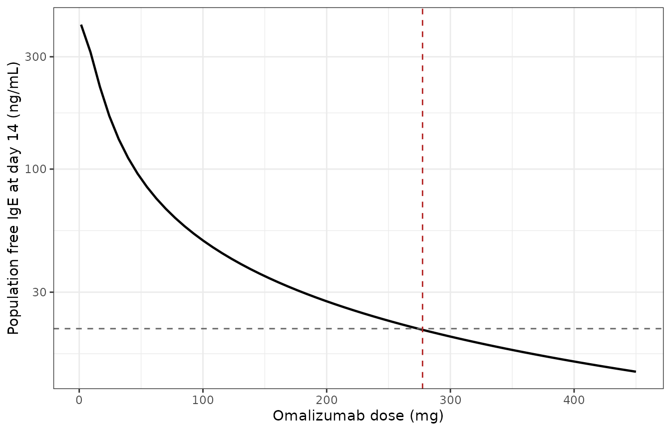

Typical-value free IgE at day 14 versus dose, replicating the black curve of Brekkan 2018 Figure 2. Horizontal line: the 21 ng/mL clinical threshold. Vertical line: the paper’s true dose of 277.5 mg.

Gate 3: the complex clearance is total, not excess

Appendix 1 Table 1A lists CLComp = 5.86 mL/h and describes it as “Complex clearance”, and equation 2 uses CL_COMP directly as the coefficient on the complex concentration. The parent Hayashi 2007 model reports the same 5.86 mL/h, but as an excess over the free-omalizumab clearance, so that the parent’s effective complex clearance is 7.32 + 5.86 = 13.18 mL/h. Both readings are defensible from the number alone, and they are not close: they differ by a factor of 2.25.

The true dose settles it. Refitting nothing and changing only that one coefficient:

cl_oma <- exp(ui$theta[["lcl"]])
cl_comp_direct <- exp(ui$theta[["lcl_complex"]])

mod_excess <- rxode2::ini(mod, lcl_complex = log(cl_oma + cl_comp_direct))
#> ℹ parameter labels from comments will be replaced by 'label()'
#> ℹ change initial estimate of `lcl_complex` to `-1.15100091955983`

dose_direct <- true_dose
dose_excess <- stats::uniroot(
  function(d) free_ige_d14(d, model = mod_excess) - target_95, interval = c(1, 1000)
)$root

arb <- data.frame(
  Reading = c("CLComp used directly (as extracted)",
              "CLComp as an excess over CLOMA (parent convention)"),
  `Complex CL (L/day)` = round(c(cl_comp_direct, cl_oma + cl_comp_direct), 4),
  `True dose (mg)` = round(c(dose_direct, dose_excess), 1),
  `Deviation from 277.5 mg (%)` =
    round(100 * (c(dose_direct, dose_excess) - 277.5) / 277.5, 1),
  check.names = FALSE
)
knitr::kable(arb)

Reading	Complex CL (L/day)	True dose (mg)	Deviation from 277.5 mg (%)
CLComp used directly (as extracted)	0.1406	271.7	-2.1
CLComp as an excess over CLOMA (parent convention)	0.3163	195.2	-29.6

stopifnot(
  # The extracted reading lands within a few percent of the paper's true dose...
  abs(100 * (dose_direct - 277.5) / 277.5) < 5,
  # ...while the excess reading is off by more than 20%, so the choice is not
  # a coin flip between two similar options.
  abs(100 * (dose_excess - 277.5) / 277.5) > 20
)

The extracted reading lands at 271.7 mg against the paper’s 277.5 mg; the excess reading lands at 195.2 mg, nearly 30% low. Appendix 1’s own table and equation are therefore taken at face value, and this model legitimately differs from modellib("Hayashi_2007_omalizumab") on this coefficient.

The reference trial design simulated

The reference design is now simulated exactly as Table 1 specifies it: 48 individuals, 12 per dose group, sampled at the 13 design times, with all IIV and residual error active. This is the data the optimal-design work is reasoning about.

A note on the event tables used throughout this vignette: doses are given on the ODE state depot, and observation rows carry cmt = "central" plus dvid = 1L. Both halves are needed. This model declares three endpoints – Cc, totalIgE and freeIgE each carry their own error model – so rxode2 maps dvid onto endpoint slots that sit after the three ODE states, and an observation row has to say which endpoint it belongs to. A bare cmt = "central" with no dvid fails with 'dvid'->'cmt' or 'cmt' on observation record. Naming the observable instead (cmt = "Cc") also runs, but it is the slot-renumbering anti-pattern that lint_vignette.R flags, and it is unnecessary: the two forms are numerically identical here (maximum absolute difference exactly 0 across all three outputs). All three analytes come back as columns on every observation row regardless, which is why a single set of observation rows yields all three profiles below.

design_times <- c(0, 0.5, 1, 2, 4, 7, 10, 14, 28, 42, 56, 70, 84)
dose_levels <- c(75, 150, 300, 375)
n_per_group <- 12L # 48 individuals / 4 dose groups (Table 1)

rxode2::rxSetSeed(20180608)

events <- do.call(rbind, lapply(seq_along(dose_levels), function(k) {
  ids <- (k - 1L) * n_per_group + seq_len(n_per_group)
  dose <- data.frame(id = ids, time = 0, amt = dose_levels[k],
                     evid = 1L, cmt = "depot", dvid = NA_integer_)
  obs <- expand.grid(id = ids, time = design_times, KEEP.OUT.ATTRS = FALSE)
  obs$amt <- NA_real_
  obs$evid <- 0L
  obs$cmt <- "central"
  obs$dvid <- 1L
  out <- rbind(dose, obs[, names(dose)])
  out$dose_mg <- dose_levels[k]
  out
}))
events <- events[order(events$id, events$time, -events$evid), ]

sim <- rxode2::rxSolve(
  mod, events,
  keep = "dose_mg", useLinCmt = FALSE, returnType = "data.frame"
)
sim$dose_lab <- factor(paste0(sim$dose_mg, " mg"),
                       levels = paste0(dose_levels, " mg"))

c(n_individuals = dplyr::n_distinct(sim$id),
  n_rows = nrow(sim),
  obs_per_individual_per_analyte = nrow(sim) / dplyr::n_distinct(sim$id))
#>                  n_individuals                         n_rows 
#>                             48                            624 
#> obs_per_individual_per_analyte 
#>                             13

stopifnot(
  dplyr::n_distinct(sim$id) == 48L,
  # 13 design times per individual, and three analytes are read off each row,
  # giving the 39 observations per individual that Table 1 counts.
  nrow(sim) == 48L * length(design_times),
  3L * nrow(sim) == 1872L,
  all(is.finite(sim$Cc)), all(is.finite(sim$totalIgE)), all(is.finite(sim$freeIgE))
)

sim |>
  select(id, time, dose_lab,
         `Total omalizumab (ug/mL)` = Cc,
         `Total IgE (ng/mL)` = totalIgE,
         `Free IgE (ng/mL)` = freeIgE) |>
  pivot_longer(-c(id, time, dose_lab), names_to = "analyte", values_to = "value") |>
  mutate(analyte = factor(analyte, levels = c("Total omalizumab (ug/mL)",
                                              "Total IgE (ng/mL)",
                                              "Free IgE (ng/mL)"))) |>
  ggplot(aes(time, value, group = id, colour = dose_lab)) +
  geom_line(alpha = 0.5) +
  facet_grid(analyte ~ dose_lab, scales = "free_y") +
  scale_y_log10() +
  labs(x = "Time (days)", y = NULL, colour = "Dose") +
  theme_bw() +
  theme(legend.position = "none")
#> Warning in scale_y_log10(): log-10 transformation introduced infinite values.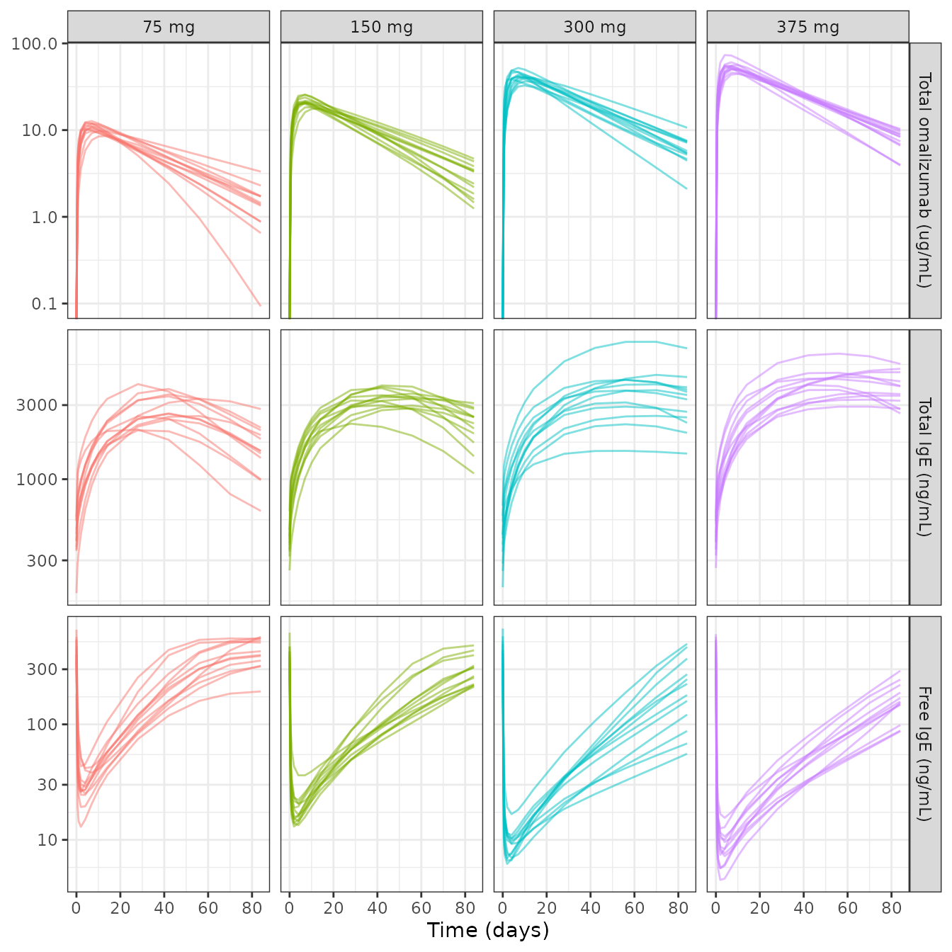

The three measured analytes over the reference design’s 84-day window, by dose group. Lines are individual profiles from the 48-subject reference design.

Free IgE falls sharply after dosing and returns toward baseline over the 84 days, total IgE rises because the complex is cleared more slowly than free IgE, and total omalizumab decays roughly log-linearly – the behaviour the paper relies on when it notes that “the measured OMA analyte was the total concentration which appeared to be linear”.

ev150 <- rbind(
  data.frame(time = 0, amt = 150, evid = 1L, cmt = "depot"),
  data.frame(time = seq(0, 84, by = 0.25), amt = NA_real_, evid = 0L, cmt = "central")
)
ev150$id <- 1L
ev150$dvid <- ifelse(ev150$evid == 0L, 1L, NA_integer_)
typ150 <- rxode2::rxSolve(
  mod, ev150, omega = NA, sigma = NA, useLinCmt = FALSE, returnType = "data.frame"
)

ggplot(typ150, aes(time, freeIgE)) +
  geom_line(linewidth = 0.8) +
  geom_hline(yintercept = baseline_closed_form, linetype = "dashed", colour = "grey40") +
  geom_hline(yintercept = 21, linetype = "dotted", colour = "firebrick") +
  scale_y_log10() +
  labs(x = "Time (days)", y = "Typical free IgE (ng/mL)") +
  theme_bw()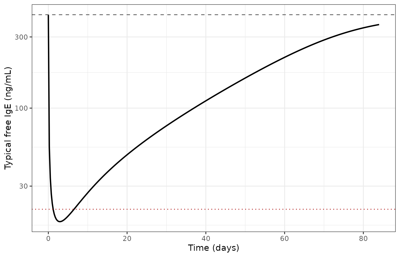

Typical-value free IgE after a 150 mg subcutaneous dose, the dose used for the population prediction areas of Brekkan 2018 Figure 3. Dashed line: pretreatment baseline. Dotted line: the 21 ng/mL threshold.

PKNCA validation of total omalizumab

Brekkan 2018 reports no non-compartmental results, so there is no published NCA table to compare against. PKNCA is used instead to test the paper’s own structural claim about this analyte: that total omalizumab “appeared to be linear” over the studied dose range. If that holds, dose-normalised AUC and Cmax must be flat across the four dose groups.

conc_data <- sim |>
  select(id, time, dose_mg, conc = Cc) |>
  filter(!is.na(conc)) |>
  mutate(treatment = factor(paste0(dose_mg, " mg"),
                            levels = paste0(dose_levels, " mg")))

dose_data <- conc_data |>
  group_by(id, treatment) |>
  summarise(dose = dplyr::first(dose_mg), time = 0, .groups = "drop")

o_conc <- PKNCA::PKNCAconc(conc_data, conc ~ time | treatment + id,
                           concu = "ug/mL", timeu = "day")
o_dose <- PKNCA::PKNCAdose(dose_data, dose ~ time | treatment + id,
                           doseu = "mg")

o_data <- PKNCA::PKNCAdata(
  o_conc, o_dose,
  intervals = data.frame(
    start = 0, end = 84,
    cmax = TRUE, tmax = TRUE, auclast = TRUE, half.life = TRUE
  )
)
res <- PKNCA::pk.nca(o_data)

nca <- as.data.frame(res) |>
  filter(PPTESTCD %in% c("cmax", "tmax", "auclast", "half.life")) |>
  left_join(distinct(conc_data, id, dose_mg), by = "id") |>
  group_by(treatment, PPTESTCD) |>
  summarise(median = median(PPORRES), dose_mg = dplyr::first(dose_mg), .groups = "drop")

nca_wide <- nca |>
  mutate(
    value = dplyr::case_when(
      PPTESTCD == "auclast" ~ median / dose_mg,
      PPTESTCD == "cmax" ~ median / dose_mg,
      TRUE ~ median
    ),
    PPTESTCD = dplyr::recode(
      PPTESTCD,
      cmax = "Cmax / dose (ug/mL per mg)",
      auclast = "AUClast / dose (ug*day/mL per mg)",
      tmax = "Tmax (day)",
      `half.life` = "t1/2 (day)"
    )
  ) |>
  select(treatment, PPTESTCD, value) |>
  pivot_wider(names_from = treatment, values_from = value) |>
  rename("NCA parameter" = PPTESTCD)

knitr::kable(nca_wide, digits = 4)

NCA parameter	75 mg	150 mg	300 mg	375 mg
AUClast / dose (ug*day/mL per mg)	5.4539	5.7797	5.6950	5.8036
Cmax / dose (ug/mL per mg)	0.1452	0.1385	0.1377	0.1430
t1/2 (day)	24.1361	25.5201	27.2350	28.5172
Tmax (day)	7.0000	7.0000	7.0000	7.0000

The linearity claim is structural, so the gate belongs on the typical-value profile rather than on medians over 12 simulated subjects per arm. A cohort median is one draw: measured across seeds and solver-thread counts the cohort spread below ranges over roughly 8-21%, which is wide enough to swallow any bound tight enough to be interesting. The same quantity computed with IIV and residual error switched off is deterministic and is what actually tests the model structure.

typ_nca <- vapply(dose_levels, function(d) {
  ev <- rbind(
    data.frame(time = 0, amt = d, evid = 1L, cmt = "depot"),
    data.frame(time = design_times, amt = NA_real_, evid = 0L, cmt = "central")
  )
  ev$id <- 1L
  ev$dvid <- ifelse(ev$evid == 0L, 1L, NA_integer_)
  s <- rxode2::rxSolve(
    mod, ev, omega = NA, sigma = NA, useLinCmt = FALSE, returnType = "data.frame"
  )
  c(cmax = max(s$Cc),
    auclast = PKNCA::pk.calc.auc(s$Cc, s$time, interval = c(0, 84), method = "linear"))
}, numeric(2))
colnames(typ_nca) <- paste0(dose_levels, " mg")

typ_dn <- sweep(typ_nca, 2, dose_levels, "/")
typ_spread <- 100 * (apply(typ_dn, 1, max) - apply(typ_dn, 1, min)) /
  apply(typ_dn, 1, median)

knitr::kable(
  data.frame(
    `NCA parameter` = c("Cmax / dose (ug/mL per mg)", "AUC0-84 / dose (ug*day/mL per mg)"),
    typ_dn,
    `Spread (%)` = round(typ_spread, 2),
    check.names = FALSE, row.names = NULL
  ),
  digits = 4
)

NCA parameter	75 mg	150 mg	300 mg	375 mg	Spread (%)
Cmax / dose (ug/mL per mg)	0.1464	0.1435	0.1420	0.1417	3.28
AUC0-84 / dose (ug*day/mL per mg)	5.7040	5.5490	5.4202	5.3874	5.77

# Cohort spread, shown for context but gated only loosely (see prose above).
dn <- nca |>
  filter(PPTESTCD %in% c("auclast", "cmax")) |>
  mutate(dosenorm = median / dose_mg) |>
  group_by(PPTESTCD) |>
  summarise(spread_pct = 100 * (max(dosenorm) - min(dosenorm)) / median(dosenorm),
            .groups = "drop")
dn
#> # A tibble: 2 × 2
#>   PPTESTCD spread_pct
#>   <chr>         <dbl>
#> 1 auclast        6.10
#> 2 cmax           5.36

stopifnot(
  # STRUCTURAL gate, deterministic: dose-normalised exposure is nearly flat
  # across the 5-fold dose range, confirming the paper's statement that the
  # measured (total) omalizumab analyte "appeared to be linear". Realised 3.3%
  # (Cmax) and 5.8% (AUC); 12 leaves headroom for solver tolerance while still
  # breaking on a mis-specified saturable term, which moves this by tens of
  # percent.
  all(typ_spread < 12),
  # Mild sub-proportionality is expected and directional: a larger fraction of
  # a small dose ends up as complex, which distributes into a smaller volume.
  all(typ_dn[, "75 mg"] > typ_dn[, "375 mg"]),
  # COHORT gate, loose. Observed 8.2 / 10.8 / 16.3 / 20.6% over seeds 20180608
  # and 99 at 2, 4 and 16 threads, so 35 sits outside the noise and still goes
  # red on a gross structural error. Do not tighten this to one observed run.
  all(dn$spread_pct < 35)
)

Dose-normalised AUC and Cmax vary by only a few percent across the 75-375 mg range on the typical-value profile, so the total-omalizumab analyte is effectively linear here, as the paper states. The small residual sub-proportionality is in the expected direction. The real nonlinearity in the system lives in the IgE arm and in free omalizumab, neither of which was measured in the reference study – which is exactly why the paper cautions that “if free OMA were measured, nonlinear PK may have been observed at certain doses”.

Assumptions and deviations

Molecular weights are not tabulated in Appendix 1. The supplement writes its ODEs in nmol but reports the go/no-go thresholds in ng/mL, so converting between the two requires molecular weights that Table 1A does not list. Both are taken from the parent Hayashi 2007 analysis (Methods, page 552): IgE 190 kDa and omalizumab 150 kDa. The IgE value is confirmed by the paper itself – ksyn / cl_ige * 190 reproduces the printed baseline of 422.82 ng/mL exactly (Gate 1). The omalizumab value is not independently confirmable from Brekkan 2018, and it is the most likely source of the residual 2.1% deviation in Gate 2: the true dose reproduces at 271.7 mg against a printed 277.5 mg, and an exact match would require 153.3 kDa, which is not a physical value for omalizumab (~149 kDa). The 150 kDa value is kept because it is the parent model’s and is sibling-consistent; it was not tuned to close the gap.
Dose units. Appendix 1’s equation 1 is written with the subcutaneous amount already in nmol. The model file doses in mg (the unit the paper’s dose groups use) and converts at the depot-to-central transfer via 1000 / MWX.
Complex clearance is used as a total, not an excess (Gate 3). This is the one coefficient on which this model deliberately differs from modellib("Hayashi_2007_omalizumab"), and the paper’s own true dose discriminates the two readings by nearly 30%.
Pretreatment total IgE is a derived initial condition. Appendix 1 gives no explicit initial condition. With the baseline-IgE covariate removed there is nothing else to set the state, and the steady state of equation 3 with no drug present reproduces the printed 422.82 ng/mL baseline, so total_target(0) = ksyn * v_ige / cl_ige is the intended reading.
No IIV on Kd0 or on VIGE. Table 1A reports omega Kd0 = 0* (fixed to zero) and lists no IIV row for VIGE. Both are carried without an eta rather than as ~ fixed(0), which would make OMEGA singular.
No covariates and no random-effect correlation, by construction. The parent model’s body-weight and baseline-IgE relationships are recorded in the model file’s covariatesDataExcluded so the provenance of the reduction is preserved; use modellib("Hayashi_2007_omalizumab") when covariate effects are wanted.
Individual count is derived, not printed: 1872 samples / 39 observations per individual = 48, corroborated by design 5’s 936 samples for two dose groups.
No NCA comparison table is rendered because Brekkan 2018 reports no non-compartmental results. The PKNCA section tests the paper’s linearity statement instead.
Not reproduced here: the design-optimization results themselves (efficiency, %RSE, PPAR and go/no-go probability for the 12 competing designs in Table 2). Those are properties of PopED / PsN optimization runs over this model, not of the model, and reproducing them is out of scope for a model validation vignette. The model this vignette ships is the reference model those results were computed from, and the true dose of Gate 2 is the one design-derived number that depends only on the model.