Dalbavancin (Carrothers 2020)
Source:vignettes/articles/Carrothers_2020_dalbavancin.Rmd
Carrothers_2020_dalbavancin.RmdModel and source
- Citation: Carrothers TJ, Chittenden JT, Critchley I. Dalbavancin Population Pharmacokinetic Modeling and Target Attainment Analysis. Clin Pharmacol Drug Dev. 2020;9(1):21-31. doi:10.1002/cpdd.695
- Description: Three-compartment intravenous population PK model for dalbavancin in adults with acute bacterial skin and skin structure infections or catheter-related bloodstream infections (pooled phase 2/3 studies VER001-4, VER001-5, VER001-9 and DUR001-303). Zero-order infusion into the central compartment and first-order elimination. Power covariate effects: albumin, creatinine clearance and body weight on CL; albumin and weight on V1; age, albumin and weight on V2; albumin and weight on V3. IIV on CL, V1, V2 and V3 as two correlated blocks (CL with V2, V1 with V3); no IIV on Q2 or Q3. Proportional residual error.
- Article (open access): https://doi.org/10.1002/cpdd.695
- Supplement (model-building trail, Tables S1-S3, Figure S1):
Supporting Information file
CPDD-9-21-s001.pdfof the same article.
Carrothers 2020 re-estimated the dalbavancin population PK model after adding the phase 3b single-dose study DUR001-303 to the three earlier phase 2/3 studies used in the prior 2-compartment analysis. Its denser early sampling supported a third compartment. The final model (supplement Run 1005) is a 3-compartment model with zero-order intravenous input, first-order elimination, power covariate effects on CL and all three volumes, two correlated IIV blocks and a proportional residual error.
Population
703 adults from four studies (Table 1, Table 2): VER001-4 (catheter-related bloodstream infection, n = 30), VER001-5 (skin and soft tissue infection, n = 34), VER001-9 (complicated skin and soft tissue infection, n = 468) and DUR001-303 (acute bacterial skin and skin structure infection, n = 171), with 2310 plasma concentrations. Pooled median (range) age 47 (18-93) years, weight 85 (43-320) kg, creatinine clearance 113 (22-440) mL/min and albumin 3.7 (1.1-5.1) g/dL; 59.2% male; 71.7% Caucasian, 14.7% Hispanic, 11.1% Black. Regimens were 1000 mg day 1 + 500 mg day 8, 1100 mg day 1, or 1500 mg single dose, with dose reduction for creatinine clearance below 30 mL/min in DUR001-303.
The same information is available programmatically via
readModelDb("Carrothers_2020_dalbavancin")()$population.
Source trace
| Equation / parameter | Value | Source location |
|---|---|---|
| Structure: 3 compartments, zero-order input, first-order elimination | - | Results, Structural Model; Figure S1; Table S1 Run 103 |
CL = CLTV (ALB/3.7)^th7 (CLCR/100)^th8 (WT/85.5)^th9 exp(eta) |
- | Covariate equation 1 under Table 3 |
V1 = V1TV (ALB/3.7)^th10 (WT/85.5)^th11 exp(eta) |
- | Covariate equation 2 under Table 3 |
V2 = V2TV (AGE/47)^th12 (ALB/3.7)^th13 (WT/85.5)^th14 exp(eta) |
- | Covariate equation 3 under Table 3 |
V3 = V3TV (ALB/3.7)^th15 (WT/85.5)^th16 exp(eta) |
- | Covariate equation 4 under Table 3 (exponents are Table 3’s theta16/theta17; see Assumptions) |
lcl |
0.0531 L/h | Table 3 theta1 |
lvc |
3.04 L | Table 3 theta2 |
lvp |
8.78 L | Table 3 theta3 |
lvp2 |
3.28 L | Table 3 theta4 |
lq (Q2, to V2) |
0.288 L/h | Table 3 theta5 |
lq2 (Q3, to V3) |
2.11 L/h | Table 3 theta6 |
e_alb_cl, e_crcl_cl,
e_wt_cl
|
-0.477, 0.273, 0.391 | Table 3 theta7-theta9 |
e_alb_vc, e_wt_vc
|
-0.340, 0.683 | Table 3 theta10-theta11 |
e_age_vp, e_alb_vp,
e_wt_vp
|
0.486, -0.413, 0.365 | Table 3 theta12-theta14 |
e_alb_vp2, e_wt_vp2
|
-0.551, 0.518 | Table 3 theta16-theta17 |
etalcl, etalvp block |
0.0489, 0.0823, 0.153 | Table 3 omega1.1, omega2.1, omega2.2; block structure from Table S3 Run 1005 |
etalvc, etalvp2 block |
0.0566, 0.111, 0.437 | Table 3 omega3.3, omega4.3, omega4.4 |
propSd |
0.190 (= sqrt(0.0362)) | Table 3 sigma1.1 (variance) |
The Table 3 omegas are log-scale variances: the printed coefficients
of variation (22%, 24%, 41%, 74%) are sqrt(omega) for CL
and sqrt(exp(omega) - 1) for V1, V2 and V3, which confirms
they are variances and not SDs. Both blocks are positive definite
(correlations 0.95 and 0.71).
mod <- readModelDb("Carrothers_2020_dalbavancin")
ref_cov <- data.frame(WT = 85.5, ALB = 37, CRCL = 100, AGE = 47)
Typical-value checks
Terminal half-life (Table 3)
Table 3 reports a terminal half-life of 8.77 days (95% CI 8.51-9.02), computed from parameter-uncertainty samples. At the reference covariates the terminal half-life is fixed by the smallest eigenvalue of the rate-constant matrix, which needs no simulation.
th <- list(cl = 0.0531, vc = 3.04, vp = 8.78, vp2 = 3.28, q = 0.288, q2 = 2.11)
kmat <- function(p) {
  with(p, matrix(c(
    -(cl + q + q2) / vc, q / vp, q2 / vp2,
    q / vc, -q / vp, 0,
    q2 / vc, 0, -q2 / vp2
  ), nrow = 3, byrow = TRUE))
}
lambda <- -eigen(kmat(th))$values
thalf_days <- log(2) / lambda / 24
thalf_days
#> [1] 0.02064091 0.36164404 8.75598635
# Deterministic identity from the published point estimates -- no sampling.
stopifnot(abs(min(lambda) * 24 / log(2) * 8.77 - 1) < 0.01)

# The same gate discriminates the Q-to-V pairing: pairing Q2 with V3 and Q3
# with V2 instead gives a clearly different terminal half-life.
th_swap <- modifyList(th, list(q = 2.11, q2 = 0.288))
log(2) / min(-eigen(kmat(th_swap))$values) / 24
#> [1] 8.355694
The printed pairing gives 8.76 days against the published 8.77, inside the 8.51-9.02 interval. The swapped pairing falls outside it. Total volume is V1 + V2 + V3 = 15.1 L, matching the abstract’s “approximately 15 L”, and CL is 0.053 L/h (abstract “0.05 L/h”).
Figure 4: population profiles of the two DUR001-303 regimens
fig4_events <- bind_rows(
  data.frame(id = 1L, treatment = "1500 mg day 1", time = 0, amt = 1500),
  data.frame(id = 2L, treatment = "1000 mg day 1 + 500 mg day 8",
             time = c(0, 168), amt = c(1000, 500))
) |>
  mutate(evid = 1L, dur = 0.5, cmt = "central")
fig4_obs <- data.frame(id = rep(1:2, each = 1),
                       treatment = c("1500 mg day 1", "1000 mg day 1 + 500 mg day 8")) |>
  tidyr::crossing(time = sort(unique(c(seq(0, 14 * 24, by = 1), seq(0, 2, by = 0.01),
                                       168 + seq(0, 2, by = 0.01))))) |>
  mutate(evid = 0L, amt = 0, dur = 0, cmt = "central")
fig4_data <- bind_rows(fig4_events, fig4_obs) |>
  cross_join(ref_cov) |>
  arrange(id, time, desc(evid))

fig4_sim <- rxSolve(zeroRe(mod), fig4_data, keep = "treatment",
                    returnType = "data.frame")
#> ℹ parameter labels from comments will be replaced by 'label()'
#> ℹ omega/sigma items treated as zero: 'etalcl', 'etalvp', 'etalvc', 'etalvp2'
#> Warning: multi-subject simulation without without 'omega'

fig4_cmax <- fig4_sim |>
  filter(time < 24) |>
  group_by(treatment) |>
  summarise(cmax = max(Cc), .groups = "drop") |>
  mutate(published = c(275.4, 413.2)[match(treatment, c("1000 mg day 1 + 500 mg day 8",
                                                        "1500 mg day 1"))])
knitr::kable(
  fig4_cmax |>
    dplyr::rename("Regimen" = treatment, "Simulated Cmax (mg/L)" = cmax,
                  "Figure 4 Cmax (mg/L)" = published),
  digits = 1,
  caption = "Typical-value first-dose Cmax at the reference covariates vs. the values printed in Figure 4."
)| Regimen | Simulated Cmax (mg/L) | Figure 4 Cmax (mg/L) |
|---|---|---|
| 1000 mg day 1 + 500 mg day 8 | 275.4 | 275.4 |
| 1500 mg day 1 | 413.1 | 413.2 |
# Deterministic (typical-value) solve against the printed labels.
stopifnot(all(abs(fig4_cmax$cmax / fig4_cmax$published - 1) < 0.01))

ggplot(fig4_sim, aes(time / 24, Cc, colour = treatment)) +
  geom_line() +
  labs(x = "Time (days)", y = "Dalbavancin concentration (mg/L)", colour = "Regimen") +
  theme_bw() +
  theme(legend.position = "top")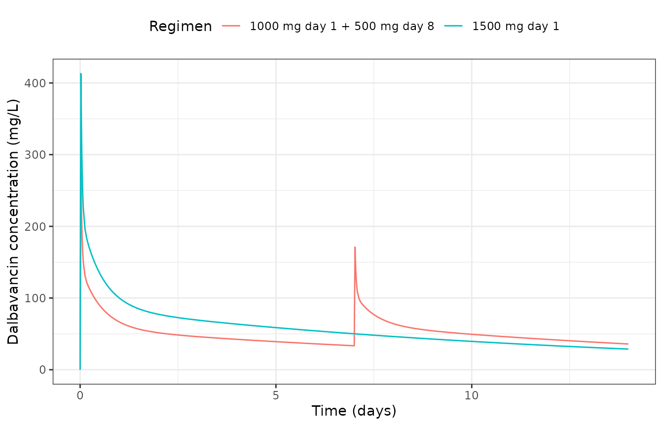
Replicates Figure 4 of Carrothers 2020. The printed Cmax labels (413.2 and 275.4 mg/L) are reproduced to within 0.1 mg/L with a 30-minute infusion at the reference covariates, which pins V1, Q3 and the infusion duration jointly.
Virtual cohort
The paper does not publish individual covariates, so a cohort is drawn from the Table 2 pooled summaries, independently for each covariate and truncated to the observed ranges: weight log-normal (median 85 kg, range 43-320), albumin normal (mean 3.7, SD 0.7 g/dL, range 1.1-5.1; supplied to the model in g/L), creatinine clearance log-normal (median 113 mL/min, range 22-440) and age normal (mean 47, SD 17 years, range 18-93). 200 subjects per regimen.
set.seed(20200101) # covariate draws (base R)
rxode2::rxSetSeed(20200101) # rxode2 eta and residual draws
n_per_arm <- 200
rtrunc <- function(n, mean, sd, lo, hi) {
  x <- numeric(0)
  while (length(x) < n) {
    y <- rnorm(n, mean, sd)
    x <- c(x, y[y >= lo & y <= hi])
  }
  x[seq_len(n)]
}
make_cohort <- function(n, id0) {
  data.frame(
    id = id0 + seq_len(n),
    WT = exp(rtrunc(n, log(85), 0.28, log(43), log(320))),
    ALB = rtrunc(n, 3.7, 0.7, 1.1, 5.1) * 10,
    CRCL = exp(rtrunc(n, log(113), 0.42, log(22), log(440))),
    AGE = rtrunc(n, 47, 17, 18, 93)
  )
}
cohort <- bind_rows(
  make_cohort(n_per_arm, 0L) |> mutate(treatment = "1500 mg day 1"),
  make_cohort(n_per_arm, n_per_arm) |> mutate(treatment = "1000 mg day 1 + 500 mg day 8")
)
cohort |>
  group_by(treatment) |>
  summarise(across(c(WT, ALB, CRCL, AGE), median), .groups = "drop") |>
knitr::kable(digits = 1, caption = "Cohort medians (ALB in g/L).")| treatment | WT | ALB | CRCL | AGE |
|---|---|---|---|---|
| 1000 mg day 1 + 500 mg day 8 | 87.1 | 36.6 | 118.6 | 47.1 |
| 1500 mg day 1 | 81.4 | 36.5 | 114.0 | 47.5 |
Simulation
doses <- bind_rows(
  cohort |> filter(treatment == "1500 mg day 1") |> mutate(time = 0, amt = 1500),
  cohort |> filter(treatment != "1500 mg day 1") |>
    tidyr::crossing(data.frame(time = c(0, 168), amt = c(1000, 500)))
) |>
  mutate(evid = 1L, dur = 0.5, cmt = "central")
obs_times <- sort(unique(c(0, 0.5, 1, 2, 4, 8, 12, 18, 24, seq(36, 120, by = 12),
                           seq(144, 28 * 24, by = 24))))
obs <- cohort |>
  tidyr::crossing(time = obs_times) |>
  mutate(evid = 0L, amt = 0, dur = 0, cmt = "central")
sim_data <- bind_rows(doses, obs) |> arrange(id, time, desc(evid))

sim <- rxSolve(mod, sim_data, keep = "treatment", returnType = "data.frame")
#> ℹ parameter labels from comments will be replaced by 'label()'

vpc <- sim |>
  filter(time > 0) |>
  group_by(treatment, time) |>
  summarise(p05 = quantile(Cc, 0.05), p50 = median(Cc), p95 = quantile(Cc, 0.95),
            .groups = "drop")
ggplot(vpc, aes(time / 24, p50)) +
  geom_ribbon(aes(ymin = p05, ymax = p95), alpha = 0.25) +
  geom_line() +
  facet_wrap(~treatment) +
  scale_y_log10() +
  labs(x = "Time (days)", y = "Dalbavancin concentration (mg/L)",
       caption = "Median and 90% prediction interval of the virtual cohort (with residual error).") +
  theme_bw()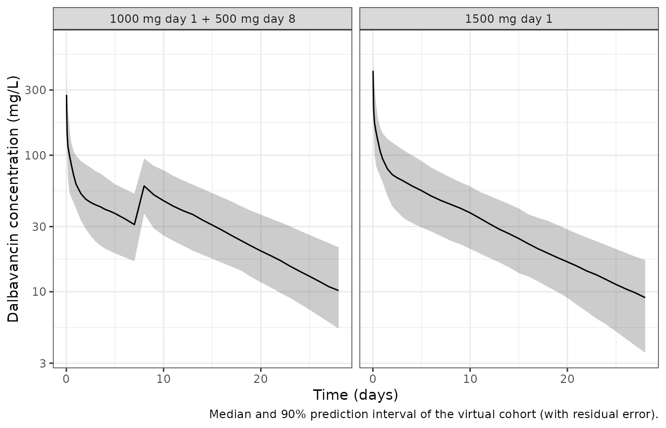
PKNCA validation
NCA of the typical-value profiles at the reference covariates, compared with the Figure 4 Cmax values and the Table 3 terminal half-life (8.77 days = 210.5 h).
nca_events <- data.frame(
  id = 1:2, treatment = c("1500 mg day 1", "1000 mg day 1"),
  time = 0, amt = c(1500, 1000), evid = 1L, dur = 0.5, cmt = "central"
)
nca_obs <- nca_events |>
  select(id, treatment) |>
  tidyr::crossing(time = sort(unique(c(0, seq(0.25, 2, by = 0.25), 4, 8, 12, 24,
                                       seq(48, 150 * 24, by = 24))))) |>
  mutate(evid = 0L, amt = 0, dur = 0, cmt = "central")
nca_data <- bind_rows(nca_events, nca_obs) |>
  cross_join(ref_cov) |>
  arrange(id, time, desc(evid))
nca_sim <- rxSolve(zeroRe(mod), nca_data, keep = "treatment",
                   returnType = "data.frame")
#> ℹ parameter labels from comments will be replaced by 'label()'
#> ℹ omega/sigma items treated as zero: 'etalcl', 'etalvp', 'etalvc', 'etalvp2'
#> Warning: multi-subject simulation without without 'omega'

sim_nca <- nca_sim |>
  filter(!is.na(Cc)) |>
  select(id, time, Cc, treatment)
sim_nca <- bind_rows(
  sim_nca,
  sim_nca |> distinct(id, treatment) |> mutate(time = 0, Cc = 0)
) |>
  distinct(id, treatment, time, .keep_all = TRUE) |>
  arrange(id, treatment, time)

conc_obj <- PKNCA::PKNCAconc(sim_nca, Cc ~ time | treatment + id)
dose_obj <- PKNCA::PKNCAdose(nca_events |> select(id, time, amt, treatment),
                             amt ~ time | treatment + id)
intervals <- data.frame(start = 0, end = Inf, cmax = TRUE, tmax = TRUE,
                        aucinf.obs = TRUE, half.life = TRUE, cl.obs = TRUE,
                        vss.obs = TRUE)
nca_res <- PKNCA::pk.nca(PKNCA::PKNCAdata(conc_obj, dose_obj, intervals = intervals))

published_nca <- tibble::tribble(
  ~treatment,       ~cmax, ~half.life, ~cl.obs, ~vss.obs,
  "1500 mg day 1",  413.2, 8.77 * 24,  0.0531,  15.1,
  "1000 mg day 1",  275.4, 8.77 * 24,  0.0531,  15.1
)
cmp_nca <- nlmixr2lib::ncaComparisonTable(
  simulated = nca_res,
  reference = published_nca,
  by = "treatment",
  units = c(cmax = "mg/L", half.life = "h", cl.obs = "L/h", vss.obs = "L"),
  tolerance_pct = 20
)
knitr::kable(
  cmp_nca,
  caption = paste("Simulated (typical value, reference covariates) vs. Carrothers 2020:",
                  "Cmax from Figure 4, t1/2 from Table 3, CL = theta1, Vss = V1 + V2 + V3.",
                  "* differs from reference by >20%.")
)| NCA parameter | treatment | Reference | Simulated | % diff |
|---|---|---|---|---|
| Cmax (mg/L) | 1500 mg day 1 | 413 | 413 | -0.0% |
| Cmax (mg/L) | 1000 mg day 1 | 275 | 275 | +0.0% |
| t½ (h) | 1500 mg day 1 | 210 | 210 | -0.2% |
| t½ (h) | 1000 mg day 1 | 210 | 210 | -0.2% |
| CL/F (L/h) | 1500 mg day 1 | 0.0531 | 0.0529 | -0.3% |
| CL/F (L/h) | 1000 mg day 1 | 0.0531 | 0.0529 | -0.3% |
| Vss/F (L) | 1500 mg day 1 | 15.1 | 15 | -0.5% |
| Vss/F (L) | 1000 mg day 1 | 15.1 | 15 | -0.5% |
nca_wide <- as.data.frame(nca_res) |>
  select(treatment, PPTESTCD, PPORRES) |>
  tidyr::pivot_wider(names_from = PPTESTCD, values_from = PPORRES)
# Typical-value solve: NCA CL and Vss of a linear model are identities of the
# parameters (CL = theta1, Vss = V1 + V2 + V3), apart from tail truncation.
stopifnot(
  all(abs(nca_wide$cl.obs / 0.0531 - 1) < 0.02),
  all(abs(nca_wide$vss.obs / 15.1 - 1) < 0.02),
  all(abs(nca_wide$half.life / (8.77 * 24) - 1) < 0.05)
)
ncaComparisonTable() labels CL and Vss as “CL/F” and
“Vss/F”; dalbavancin is given intravenously, so F = 1.
Probability of target attainment (Figure 5)
The paper computes the daily average free AUC as
fu * AUC(0-120 h) / 5 with fu = 0.07 (Methods)
after a 1500 mg single dose, and reports target attainment against the
murine-thigh targets fAUC/MIC = 27.1 (stasis), 53.3 (1-log kill), 111.1
(2-log kill) and the superseded stasis target of 265 (Results, Target
Attainment).
auc120 <- sim |>
  filter(treatment == "1500 mg day 1", time <= 120) |>
  arrange(id, time) |>
  group_by(id) |>
  summarise(auc = sum(diff(time) * (head(Cc, -1) + tail(Cc, -1)) / 2), .groups = "drop")

pta <- tidyr::crossing(target = c(27.1, 53.3, 111.1, 265),
                       mic = c(0.125, 0.25, 0.5, 1, 2, 4, 8)) |>
  rowwise() |>
  mutate(pta = 100 * mean(0.07 * auc120$auc / 5 / mic >= target)) |>
  ungroup()

published_pta <- tibble::tribble(
  ~target, ~mic, ~published,
  27.1,    2,    "99",
  27.1,    4,    "87.7",
  53.3,    1,    "99",
  111.1,   0.5,  "99",
  265,     0.25, ">99",
  265,     0.5,  "65"
)
knitr::kable(
  published_pta |>
    left_join(pta, by = c("target", "mic")) |>
    dplyr::rename("fAUC/MIC target" = target, "MIC (mg/L)" = mic,
                  "Published PTA (%)" = published, "Simulated PTA (%)" = pta),
  digits = c(1, 3, 0, 1),
  caption = "Target attainment for 1500 mg single dose, Carrothers 2020 Results and Figure 5."
)| fAUC/MIC target | MIC (mg/L) | Published PTA (%) | Simulated PTA (%) |
|---|---|---|---|
| 27.1 | 2.00 | 99 | 100.0 |
| 27.1 | 4.00 | 87.7 | 82.0 |
| 53.3 | 1.00 | 99 | 100.0 |
| 111.1 | 0.50 | 99 | 100.0 |
| 265.0 | 0.25 | >99 | 99.5 |
| 265.0 | 0.50 | 65 | 57.0 |
ggplot(pta, aes(mic, pta, colour = factor(target))) +
  geom_line() +
  geom_point() +
  scale_x_log10() +
  labs(x = "MIC (mg/L)", y = "Target attainment (%)", colour = "fAUC/MIC target") +
  theme_bw()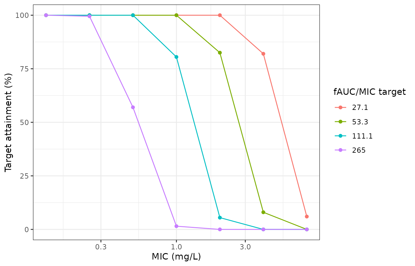
pta_at <- function(tg, m) pta$pta[pta$target == tg & pta$mic == m]
# Bands, not points: the PTA is a tail probability of a random 200-subject
# cohort (Monte Carlo SE ~3 points near 65%), and the paper resampled
# empirical-Bayes estimates of its own 703 subjects rather than a synthetic
# cohort. The bands still fail on a 2-fold error in CL, dose or fu.
stopifnot(
  pta_at(27.1, 2) > 90,
  pta_at(27.1, 4) > 65, pta_at(27.1, 4) < 97,
  pta_at(265, 0.5) > 40, pta_at(265, 0.5) < 85,
  pta_at(265, 0.25) > 90
)
Replicates the target-attainment line of Figure 5 and the PTA values quoted in Results. At the four printed values near 99-100% the simulation agrees. At the two mid-range values (stasis target at MIC 4 mg/L, old target at MIC 0.5 mg/L) the simulated PTA is 6-8 points lower (about 82% vs 87.7% and 57% vs 65% with this seed). This means the synthetic cohort’s AUC(0-120) distribution sits somewhat below the paper’s in its central quantiles (about 7-9% in an exploratory 1000-subject draw). The likely causes are (a) the independent, uncorrelated covariate draws, and (b) the paper resampling empirical-Bayes parameters, which shrinkage pulls towards the typical value. The typical-value checks above reproduce the published numbers to within 0.5%. The parameters are not tuned.
Assumptions and deviations
- V3 exponent numbering. The printed V3 equation uses theta15 (ALB) and theta16 (WT), while Table 3 lists V3-ALB as theta16 and V3-WT as theta17 and has no theta15. The values are mapped by the covariate NAME in Table 3, which is unambiguous. The missing theta15 is consistent with the age-on-V3 effect that the supplement (Table S3, Run 1003) removed.
-
Albumin units. The paper uses g/dL (reference 3.7).
The model takes canonical g/L and converts inline
(
alb_gdL <- ALB * 0.1). -
Creatinine clearance. The estimating equation is
not stated in the paper or supplement, and there is no sign of BSA
normalisation. It is encoded as raw mL/min in
CRCLwith reference 100 mL/min. Table 2’s unit label “mg/mL” is a misprint. The authors caution against simulating below 30 mL/min. - Q-to-V pairing. Table 3 names Q2 and Q3 without explicitly stating which peripheral volume each connects to. Q2 is paired with V2 and Q3 with V3. This is the pairing that reproduces both the Figure 4 Cmax labels and the Table 3 half-life; the swapped pairing fails both.
- Virtual cohort. Covariates are drawn independently from Table 2 summaries, with no correlation structure, because individual data are not published. The paper instead resampled the empirical-Bayes parameters of its own subjects for the PTA. Its PTA values are therefore compared only against bands.
-
Protein binding.
fu = 0.07is applied in the vignette’s PTA only. The model predicts total plasma concentration. - Exposure-response. The paper’s logistic regressions (Figure 3) found no exposure-response relationship (all P >= 0.33) and report no coefficients beyond near-zero figure slopes. No PD model is extracted.