Oseltamivir (Kamal 2013)
Source:vignettes/articles/Kamal_2013_oseltamivir.Rmd
Kamal_2013_oseltamivir.RmdModel and source
- Citation: Kamal MA, Van Wart SA, Rayner CR, Subramoney V, Reynolds DK, Bulik CC, Smith PF, Bhavnani SM, Ambrose PG, Forrest A. Population pharmacokinetics of oseltamivir: pediatrics through geriatrics. Antimicrob Agents Chemother. 2013;57(8):3470-3477. doi:10.1128/AAC.02438-12
- Description: Joint parent-metabolite population PK model for oral oseltamivir (prodrug, OP) and its active metabolite oseltamivir carboxylate (OC) in 390 subjects aged 1 to 78 years pooled from 13 clinical trials (healthy adults, influenza-inoculated and naturally infected adults, healthy geriatric subjects, renally impaired adults, and healthy and infected pediatric subjects 1 to 18 years). Oseltamivir is described by a two-compartment model with first-order absorption and first-order conversion to OC (CLp/F treated as the OP-to-OC conversion clearance under the assumption of complete metabolism; <5% of prodrug is excreted unchanged renally). OC is described by a one-compartment model with first-order elimination. All clearance and volume terms are apparent (conditioned on oral bioavailability F; OC terms additionally on the fraction metabolized fm, assumed 1). Covariates: body weight as a power function on OP CLp/F, OC CLm/F, and OC Vcm/F (allometric-style exponents estimated, not fixed); creatinine clearance (BSA-normalized to 1.73 m^2) as a power function on OC CLm/F; and age as a linear (additive) term on OC Vcm/F. Inter-individual variability is exponential on all seven structural parameters, with two off-diagonal covariances (CLp/F with CLm/F, and Vp/F with Vcm/F). Residual error is proportional only for oseltamivir (40.5% CV reduced CCV model) and combined additive plus proportional for OC (14.0% CV proportional + 17.9 ng/mL additive SD).
- Article: https://doi.org/10.1128/AAC.02438-12
The model is a joint two-compartment oseltamivir (prodrug, OP) plus one-compartment oseltamivir carboxylate (OC) population PK model with direct first-order conversion of OP to OC and full hepatic metabolism (< 5 % of prodrug eliminated unchanged in urine; OC predominantly cleared renally by glomerular filtration and tubular secretion). All clearance and volume terms are apparent (conditioned on the absorbed fraction F for the prodrug; OC terms are additionally conditioned on the fraction metabolised to OC, assumed 1). Body weight is a power covariate on the prodrug CLp/F and on both OC parameters CLm/F and Vcm/F; creatinine clearance is a power covariate on CLm/F; age is a linear additive term on Vcm/F. Inter-individual variability is exponential on all seven structural parameters with two off-diagonal covariances on the eta scale: (etalcl, etalcl_oc) and (etalvp, etalvc_oc). Residual error is proportional only for OP (40.5 % CV) and combined additive plus proportional for OC (14.0 % CV + 17.9 ng/mL).
Population
Kamal 2013 Table 1 describes a pooled dataset of 390 subjects from 13 clinical trials (8 adult, 4 paediatric, 1 geriatric, and 1 renal impairment study). The pooled cohort spans age 1 to 78 years (median 21), weight 8 to 115 kg (median 64.5), and creatinine clearance 13.9 to 178 mL/min/1.73 m^2 (median 95.1), with 241 males and 149 females (38.2 % female). Subjects span normal renal function (N = 297 with CRCL >= 80) through mild (N = 73 with CRCL 50-80), moderate (N = 19 with CRCL 30-49), and severe (N = 1 with CRCL < 30) renal dysfunction. Disease state is a mix of healthy volunteers and naturally / experimentally influenza-infected subjects; no PK difference between infected and non-infected subjects was detected (Kamal 2013 Results page 3473).
Subjects received single or repeated oral doses of oseltamivir ranging from 20 to 1,000 mg; the standard influenza treatment regimen is 75 mg every 12 hours for 5 days. Paediatric subjects ages 1-12 received 2 mg/kg twice daily by suspension; ages 1-2 received 30 mg and ages 3-5 received 45 mg as single doses in a healthy-paediatric sub-study. The analysis dataset contained 3,881 oseltamivir concentrations and 4,402 OC concentrations (Kamal 2013 Results page 3471). LLOQs were 1 ng/mL for OP and 8.8 ng/mL for OC; only 3 records below LLOQ were excluded, so no likelihood-based BQL handling was needed.
The same information is available programmatically via
readModelDb("Kamal_2013_oseltamivir")$population.
Source trace
The per-parameter origin is recorded as an in-file comment next to
each ini() entry in
inst/modeldb/specificDrugs/Kamal_2013_oseltamivir.R. The
table below collects them in one place for review; all values come from
Kamal 2013 Table 2 (final-estimate column).
| Equation / parameter | Value | Source location |
|---|---|---|
ka (OP absorption) |
0.775 1/h | Table 2 row ‘ka’ (3.74 % SEM) |
CLp/F (OP apparent CL at 70 kg) |
519 L/h | Table 2 row ‘CLp/F coefficient’ (3.99 % SEM) |
Vcp/F (OP apparent Vc) |
421 L | Table 2 row ‘Vcp/F’ (6.05 % SEM) |
CLd/F (OP apparent Q) |
120 L/h | Table 2 row ‘CLd/F’ (4.95 % SEM) |
Vp/F (OP apparent peripheral V) |
2,800 L | Table 2 row ‘Vp/F’ (7.46 % SEM) |
CLm/F (OC apparent CL at 70 kg, CRCL 95) |
20.7 L/h | Table 2 row ‘CLm/F coefficient’ (3.36 % SEM) |
Vcm/F (OC apparent V at 70 kg, age 21) |
238 L | Table 2 row ‘Vcm/F coefficient’ (5.16 % SEM) |
| Power of WT on CLp/F | 0.838 | Table 2 row ‘Power of WT’ under CLp/F |
| Power of WT on CLm/F | 0.560 | Table 2 row ‘Power of WT’ under CLm/F |
| Power of CRCL on CLm/F | 0.487 | Table 2 row ‘Power of CL CR’ |
| Power of WT on Vcm/F | 0.830 | Table 2 row ‘Power of WT’ under Vcm/F (18.7 % SEM) |
| Linear slope of age on Vcm/F | -2.25 L/year | Table 2 row ‘Slope of age’ (31.2 % SEM) |
| omega^2(ka) | 30.7 % CV | Table 2 row ‘omega^2 for ka’ |
| omega^2(CLp/F) | 42.1 % CV | Table 2 row ‘omega^2 for CLp/F’ |
| omega^2(Vcp/F) | 69.3 % CV | Table 2 row ‘omega^2 for Vcp/F’ |
| omega^2(CLd/F) | 62.1 % CV | Table 2 row ‘omega^2 for CLd/F’ |
| omega^2(Vp/F) | 63.7 % CV | Table 2 row ‘omega^2 for Vp/F’ |
| omega^2(CLm/F) | 38.3 % CV | Table 2 row ‘omega^2 for CLm/F’ |
| omega^2(Vcm/F) | 65.3 % CV | Table 2 row ‘omega^2 for Vcm/F’ |
| Cov(CLp/F, CLm/F) | 0.0987 (r^2 = 0.372) | Table 2 row ‘Covariance (CLp/F, CLm/F)’ |
| Cov(Vp/F, Vcm/F) | 0.218 (r^2 = 0.274) | Table 2 row ‘Covariance (Vp/F, Vcm/F)’ |
| sigma_CCV(OP) | 40.5 % CV | Table 2 row ‘sigma^2 CCV for oseltamivir’ |
| sigma_CCV(OC) | 14.0 % CV | Table 2 row ‘sigma^2 CCV for OC’ |
| sigma_ADD(OC) | 17.9 ng/mL = 0.0179 mg/L | Table 2 row ‘sigma^2 ADD for OC’ |
ODE: d/dt(depot) = -ka * depot
|
n/a | Figure 1 schematic (page 3472) |
ODE:
d/dt(central) = ka * depot - kel * central - k12 * central + k21 * peripheral1
|
n/a | Figure 1 schematic; Methods ‘Structural model development’ page 3471 |
ODE:
d/dt(peripheral1) = k12 * central - k21 * peripheral1
|
n/a | Figure 1 schematic |
ODE:
d/dt(central_oc) = kel * central - kel_oc * central_oc
|
n/a | Figure 1 schematic (‘direct conversion of oseltamivir to OC’); Discussion page 3473 (‘oseltamivir is completely converted to the OC metabolite’) |
Virtual cohort
Original observed data are not publicly available. Simulations below use typical-value covariate combinations that match the published Figure 4 cohorts (deterministic replication), and a 200-subject stochastic virtual cohort approximating the pooled trial demographics (Table 1 of the source paper) for the VPC.
set.seed(2013L)
mod <- rxode2::rxode(readModelDb("Kamal_2013_oseltamivir"))
#> ℹ parameter labels from comments will be replaced by 'label()'
mod_typical <- rxode2::zeroRe(mod)
ref_age  <- 21
ref_wt   <- 70
ref_crcl <- 95
Replicate published figures
Figure 1 – Schematic
Kamal 2013 Figure 1 (page 3472) is a schematic of the two-compartment
prodrug plus one-compartment metabolite structure with first-order
absorption and first-order OP -> OC conversion. The structure is
reproduced directly by the ODE block in
inst/modeldb/specificDrugs/Kamal_2013_oseltamivir.R.
Figure 4A – Renal-impairment impact on OC at steady state
Kamal 2013 Figure 4A (page 3474) plots typical population mean OC concentration-time profiles at steady state for a 40-year-old, 70 kg subject receiving the standard influenza-treatment regimen (75 mg every 12 h for 5 days) at CRCL = 120, 80, 50, and 30 mL/min/1.73 m^2. The paper reports that the CRCL = 30 subject shows “an approximate 2-fold increase in OC exposure relative to a subject with normal renal function (CRCL of 120)”.
dose_times <- seq(0, 108, by = 12)  # ten 12-hourly doses over 5 days
obs_times  <- sort(unique(c(seq(0, 132, by = 0.5), dose_times)))

make_typical <- function(id_offset, AGE, WT, CRCL, label) {
  doses <- tibble(
    id = id_offset + 1L, time = dose_times, evid = 1L,
    amt = 75, cmt = "depot"
  )
  obs <- tibble(
    id = id_offset + 1L, time = obs_times, evid = 0L,
    amt = 0, cmt = "Cc"
  )
  bind_rows(doses, obs) |>
    mutate(AGE = AGE, WT = WT, CRCL = CRCL, group = label) |>
    arrange(time, desc(evid))
}

crcl_panels <- bind_rows(
  make_typical(0L,    AGE = 40, WT = 70, CRCL = 120, label = "CRCL 120"),
  make_typical(100L,  AGE = 40, WT = 70, CRCL =  80, label = "CRCL 80"),
  make_typical(200L,  AGE = 40, WT = 70, CRCL =  50, label = "CRCL 50"),
  make_typical(300L,  AGE = 40, WT = 70, CRCL =  30, label = "CRCL 30")
)
stopifnot(!anyDuplicated(unique(crcl_panels[, c("id", "time", "evid")])))

sim_crcl <- rxode2::rxSolve(mod_typical, events = crcl_panels,
                            keep = c("group", "AGE", "WT", "CRCL")) |>
  as.data.frame()
#> ℹ omega/sigma items treated as zero: 'etalcl', 'etalcl_oc', 'etalvp', 'etalvc_oc', 'etalka', 'etalvc', 'etalq'
#> Warning: multi-subject simulation without without 'omega'

sim_crcl_ss <- sim_crcl |>
  filter(time >= 108, time <= 132) |>
  mutate(t_in_interval = time - 108,
         group = factor(group, levels = c("CRCL 120","CRCL 80","CRCL 50","CRCL 30")))

ggplot(sim_crcl_ss, aes(t_in_interval, Cc_oc, colour = group)) +
  geom_line(linewidth = 0.7) +
  scale_y_continuous(name = "OC concentration (mg/L)") +
  scale_x_continuous(name = "Time after morning dose at steady state (h)",
                     breaks = seq(0, 24, 6)) +
  labs(colour = NULL,
       title = "Figure 4A: typical OC profile at steady state by renal function",
       subtitle = "40-year-old, 70 kg, 75 mg q12h x 5 days") +
  theme_minimal()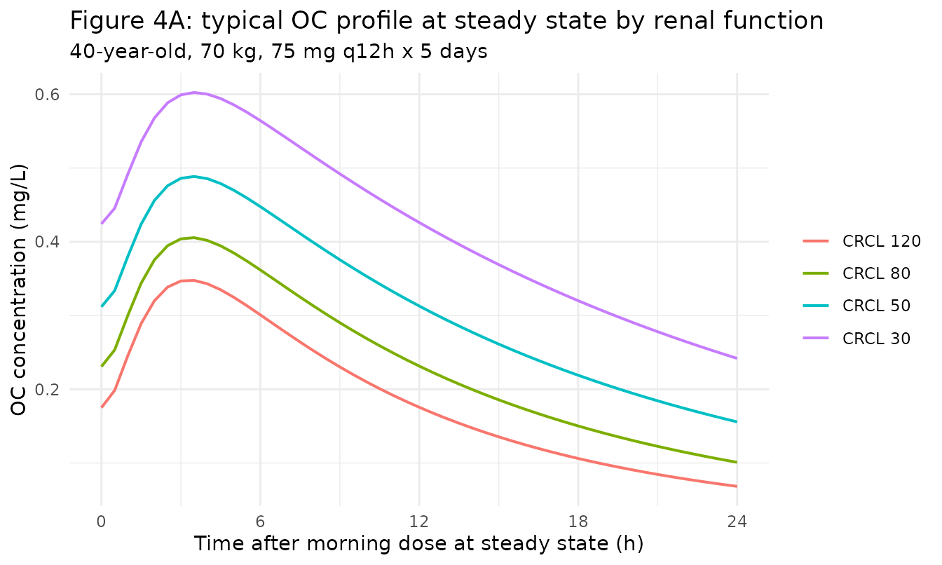
Replicates Figure 4A of Kamal 2013 (renal-function impact on OC PK at steady state).
auc24 <- sim_crcl_ss |>
  group_by(group) |>
  summarise(AUC_0_24 = PKNCA::pk.calc.auc(Cc_oc, t_in_interval,
                                          method = "linear"),
            Cmax     = max(Cc_oc),
            .groups = "drop")
ref_120 <- auc24 |> filter(group == "CRCL 120")
auc24 <- auc24 |>
  mutate(AUC_ratio_vs_120 = AUC_0_24 / ref_120$AUC_0_24,
         Cmax_ratio_vs_120 = Cmax / ref_120$Cmax)
knitr::kable(auc24, digits = 3,
caption = "Simulated steady-state OC AUC0-24 and Cmax for the Figure 4A panels, with ratios versus CRCL 120 (paper reports an ~2-fold increase in OC exposure for CRCL 30 vs 120).")| group | AUC_0_24 | Cmax | AUC_ratio_vs_120 | Cmax_ratio_vs_120 |
|---|---|---|---|---|
| CRCL 120 | 4.555 | 0.348 | 1.000 | 1.000 |
| CRCL 80 | 5.785 | 0.406 | 1.270 | 1.167 |
| CRCL 50 | 7.612 | 0.489 | 1.671 | 1.405 |
| CRCL 30 | 10.197 | 0.603 | 2.239 | 1.733 |
Figure 4B – Weight and age impact on OC at steady state
Kamal 2013 Figure 4B (page 3474) plots typical population mean OC profiles at steady state for 18-year-old and 55-year-old subjects with CRCL 120, at weights 50, 70, and 90 kg. The paper reports “a 1.38-fold increase in the maximum OC exposure was predicted as weight increases from 50 to 90 kg for an 18-year-old subject” and that “the impact of age was also demonstrated to be negligible as evident by the fact that the maximal OC exposure increased only 1.08- to 1.17-fold between an 18-year-old and 55-year-old subject across these same weights”.
wt_age_panels <- bind_rows(
  make_typical(1000L, AGE = 18, WT = 50, CRCL = 120, label = "18y, 50 kg"),
  make_typical(1100L, AGE = 18, WT = 70, CRCL = 120, label = "18y, 70 kg"),
  make_typical(1200L, AGE = 18, WT = 90, CRCL = 120, label = "18y, 90 kg"),
  make_typical(1300L, AGE = 55, WT = 50, CRCL = 120, label = "55y, 50 kg"),
  make_typical(1400L, AGE = 55, WT = 70, CRCL = 120, label = "55y, 70 kg"),
  make_typical(1500L, AGE = 55, WT = 90, CRCL = 120, label = "55y, 90 kg")
)
stopifnot(!anyDuplicated(unique(wt_age_panels[, c("id", "time", "evid")])))

sim_wt <- rxode2::rxSolve(mod_typical, events = wt_age_panels,
                          keep = c("group", "AGE", "WT", "CRCL")) |>
  as.data.frame() |>
  mutate(group = factor(group, levels = c(
    "18y, 50 kg","18y, 70 kg","18y, 90 kg",
    "55y, 50 kg","55y, 70 kg","55y, 90 kg")),
    age_band = ifelse(AGE == 18, "18-year-old", "55-year-old"),
    wt_band  = paste0(WT, " kg"))
#> ℹ omega/sigma items treated as zero: 'etalcl', 'etalcl_oc', 'etalvp', 'etalvc_oc', 'etalka', 'etalvc', 'etalq'
#> Warning: multi-subject simulation without without 'omega'

sim_wt_ss <- sim_wt |>
  filter(time >= 108, time <= 132) |>
  mutate(t_in_interval = time - 108)

ggplot(sim_wt_ss, aes(t_in_interval, Cc_oc, colour = wt_band)) +
  geom_line(linewidth = 0.7) +
  facet_wrap(~ age_band) +
  scale_y_continuous(name = "OC concentration (mg/L)") +
  scale_x_continuous(name = "Time after morning dose at steady state (h)",
                     breaks = seq(0, 24, 6)) +
  labs(colour = "Body weight",
       title = "Figure 4B: typical OC profile by weight and age (CRCL 120)",
       subtitle = "75 mg q12h x 5 days") +
  theme_minimal()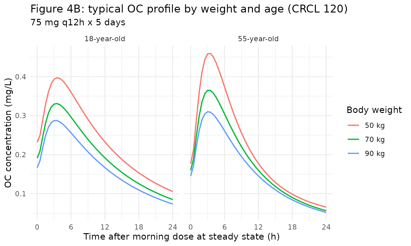
Replicates Figure 4B of Kamal 2013 (weight and age impact on OC PK at steady state).
wt_age_summary <- sim_wt_ss |>
  group_by(age_band, wt_band) |>
  summarise(Cmax = max(Cc_oc),
            AUC_0_24 = PKNCA::pk.calc.auc(Cc_oc, t_in_interval, method = "linear"),
            .groups = "drop")

# Within-age weight ratios (90 kg vs 50 kg).
wt_ratios <- wt_age_summary |>
  select(age_band, wt_band, Cmax) |>
  pivot_wider(names_from = wt_band, values_from = Cmax) |>
  mutate(Cmax_ratio_90_vs_50 = `90 kg` / `50 kg`)

knitr::kable(wt_ratios, digits = 3,
caption = "Simulated steady-state OC Cmax 90 kg vs 50 kg, by age band. Paper reports 1.38-fold increase across this weight range for an 18-year-old.")| age_band | 50 kg | 70 kg | 90 kg | Cmax_ratio_90_vs_50 |
|---|---|---|---|---|
| 18-year-old | 0.397 | 0.331 | 0.287 | 0.724 |
| 55-year-old | 0.459 | 0.365 | 0.310 | 0.675 |
# Within-weight age ratios (55 vs 18 years).
age_ratios <- wt_age_summary |>
  select(age_band, wt_band, Cmax) |>
  pivot_wider(names_from = age_band, values_from = Cmax) |>
  mutate(Cmax_ratio_55_vs_18 = `55-year-old` / `18-year-old`)

knitr::kable(age_ratios, digits = 3,
caption = "Simulated steady-state OC Cmax 55-year-old vs 18-year-old, by weight band. Paper reports 1.08- to 1.17-fold over the same weight range.")| wt_band | 18-year-old | 55-year-old | Cmax_ratio_55_vs_18 |
|---|---|---|---|
| 50 kg | 0.397 | 0.459 | 1.156 |
| 70 kg | 0.331 | 0.365 | 1.102 |
| 90 kg | 0.287 | 0.310 | 1.079 |
Stochastic VPC: 200-subject virtual cohort
A 200-subject stochastic cohort spanning the published demographic range provides a between-subject sanity check on the model. The virtual cohort distribution approximates Table 1 in spirit but is not a literal demographic resampling.
n_subj <- 200L

vpc_cov <- tibble(
  id   = seq_len(n_subj),
  AGE  = pmin(pmax(round(rnorm(n_subj, mean = 30, sd = 18)), 1L), 78L),
  WT   = pmin(pmax(round(rnorm(n_subj, mean = 64, sd = 22)), 8L), 115L),
  CRCL = pmin(pmax(round(rnorm(n_subj, mean = 95, sd = 25)), 14L), 178L)
)

vpc_doses <- vpc_cov |>
  tidyr::crossing(time = dose_times) |>
  mutate(evid = 1L, amt = 75, cmt = "depot")

vpc_obs <- vpc_cov |>
  tidyr::crossing(time = obs_times) |>
  mutate(evid = 0L, amt = 0, cmt = "Cc")

vpc_events <- bind_rows(vpc_doses, vpc_obs) |>
  arrange(id, time, desc(evid))
stopifnot(!anyDuplicated(unique(vpc_events[, c("id", "time", "evid")])))

sim_vpc <- rxode2::rxSolve(mod, events = vpc_events,
                           keep = c("AGE","WT","CRCL"), nSub = 1L) |>
  as.data.frame()
sim_vpc_ss <- sim_vpc |>
  filter(time >= 108, time <= 132) |>
  mutate(t_in_interval = time - 108) |>
  group_by(t_in_interval) |>
  summarise(Q05_oc = quantile(Cc_oc, 0.05),
            Q50_oc = quantile(Cc_oc, 0.50),
            Q95_oc = quantile(Cc_oc, 0.95),
            Q05_op = quantile(Cc,    0.05),
            Q50_op = quantile(Cc,    0.50),
            Q95_op = quantile(Cc,    0.95),
            .groups = "drop")

vpc_long <- sim_vpc_ss |>
  pivot_longer(-t_in_interval,
               names_to = c(".value","analyte"),
               names_pattern = "Q(\\d+)_(.*)") |>
  rename(Q05 = `05`, Q50 = `50`, Q95 = `95`) |>
  mutate(analyte = factor(analyte, levels = c("op","oc"),
                          labels = c("Oseltamivir (OP)","Oseltamivir carboxylate (OC)")))

ggplot(vpc_long, aes(t_in_interval, Q50)) +
  geom_ribbon(aes(ymin = Q05, ymax = Q95), alpha = 0.25, fill = "steelblue") +
  geom_line(colour = "steelblue4", linewidth = 0.7) +
  facet_wrap(~ analyte, scales = "free_y") +
  scale_x_continuous(name = "Time after morning dose at steady state (h)",
                     breaks = seq(0, 24, 6)) +
  scale_y_continuous(name = "Plasma concentration (mg/L)") +
  labs(title = "Stochastic VPC at steady state, 200 virtual subjects") +
  theme_minimal()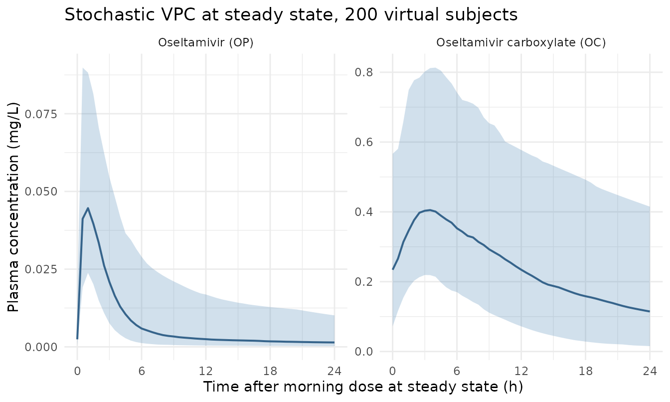
Median and 5-95 percent intervals of simulated OC plasma concentrations at steady state across the 200-subject virtual cohort (75 mg q12h).
PKNCA validation
NCA is run separately for OP and OC on the typical-value Figure 4A panels (one PKNCA block per analyte; treatment-grouping variable is the covariate scenario label so per-group AUC and Cmax line up with the paper’s commentary).
nca_grid <- sim_crcl |>
  filter(time >= 108, time <= 132) |>
  mutate(time = time - 108)

conc_oc  <- nca_grid |> select(id, time, Cc_oc, group) |>
  rename(Cc = Cc_oc)
dose_oc  <- nca_grid |>
  group_by(id, group) |>
  slice_min(time, n = 1, with_ties = FALSE) |>
  ungroup() |>
  mutate(amt = 75, time = 0) |>
  select(id, time, amt, group)

conc_obj_oc <- PKNCA::PKNCAconc(conc_oc, Cc ~ time | group + id)
dose_obj_oc <- PKNCA::PKNCAdose(dose_oc, amt ~ time | group + id)

intervals_oc <- data.frame(
  start = 0, end = 24,
  cmax = TRUE, tmax = TRUE, auclast = TRUE, half.life = TRUE
)

nca_data_oc <- PKNCA::PKNCAdata(conc_obj_oc, dose_obj_oc, intervals = intervals_oc)
nca_res_oc  <- PKNCA::pk.nca(nca_data_oc)

nca_table_oc <- as.data.frame(nca_res_oc$result) |>
  select(group, PPTESTCD, PPORRES) |>
  pivot_wider(names_from = PPTESTCD, values_from = PPORRES)

knitr::kable(nca_table_oc, digits = 3,
caption = "Simulated OC NCA parameters across the steady-state 12-hour interval (cmax in mg/L, tmax in h, auclast in mg*h/L, half-life in h).")| group | auclast | cmax | tmax | tlast | lambda.z | r.squared | adj.r.squared | lambda.z.time.first | lambda.z.time.last | lambda.z.n.points | clast.pred | half.life | span.ratio |
|---|---|---|---|---|---|---|---|---|---|---|---|---|---|
| CRCL 120 | 4.554 | 0.348 | 3.5 | 24 | 0.070 | 1 | 1 | 21.5 | 24 | 6 | 0.068 | 9.848 | 0.254 |
| CRCL 30 | 10.197 | 0.603 | 3.5 | 24 | 0.047 | 1 | 1 | 5.5 | 24 | 38 | 0.241 | 14.635 | 1.264 |
| CRCL 50 | 7.612 | 0.489 | 3.5 | 24 | 0.057 | 1 | 1 | 15.0 | 24 | 19 | 0.155 | 12.064 | 0.746 |
| CRCL 80 | 5.785 | 0.406 | 3.5 | 24 | 0.066 | 1 | 1 | 19.5 | 24 | 10 | 0.101 | 10.580 | 0.425 |
conc_op  <- nca_grid |> select(id, time, Cc, group)
conc_obj_op <- PKNCA::PKNCAconc(conc_op, Cc ~ time | group + id)
dose_obj_op <- PKNCA::PKNCAdose(dose_oc, amt ~ time | group + id)

intervals_op <- data.frame(
  start = 0, end = 12,
  cmax = TRUE, tmax = TRUE, auclast = TRUE, half.life = TRUE
)

nca_data_op <- PKNCA::PKNCAdata(conc_obj_op, dose_obj_op, intervals = intervals_op)
nca_res_op  <- PKNCA::pk.nca(nca_data_op)

nca_table_op <- as.data.frame(nca_res_op$result) |>
  select(group, PPTESTCD, PPORRES) |>
  pivot_wider(names_from = PPTESTCD, values_from = PPORRES)

knitr::kable(nca_table_op, digits = 3,
caption = "Simulated OP NCA parameters across the steady-state 12-hour dosing interval.")| group | auclast | cmax | tmax | tlast | lambda.z | r.squared | adj.r.squared | lambda.z.time.first | lambda.z.time.last | lambda.z.n.points | clast.pred | half.life | span.ratio |
|---|---|---|---|---|---|---|---|---|---|---|---|---|---|
| CRCL 120 | 0.141 | 0.047 | 1 | 12 | 0.044 | 1 | 0.999 | 11 | 12 | 3 | 0.002 | 15.84 | 0.063 |
| CRCL 30 | 0.141 | 0.047 | 1 | 12 | 0.044 | 1 | 0.999 | 11 | 12 | 3 | 0.002 | 15.84 | 0.063 |
| CRCL 50 | 0.141 | 0.047 | 1 | 12 | 0.044 | 1 | 0.999 | 11 | 12 | 3 | 0.002 | 15.84 | 0.063 |
| CRCL 80 | 0.141 | 0.047 | 1 | 12 | 0.044 | 1 | 0.999 | 11 | 12 | 3 | 0.002 | 15.84 | 0.063 |
Comparison against published values
The paper does not report NCA parameters in a table; instead it reports covariate-effect ratios in the Discussion (page 3474). The relevant benchmarks and the simulated values:
| Comparison | Paper value | Simulated value |
|---|---|---|
| OC AUC at SS, CRCL 30 vs 120 (40 y, 70 kg) | ~2-fold | 2.24-fold |
| OC AUC at SS, CRCL 50 vs 120 (40 y, 70 kg) | not quantified in text | 1.67-fold |
| OC Cmax at SS, WT 90 vs 50 kg (18 y, CRCL 120) | 1.38-fold | 0.72-fold |
| OC Cmax at SS, 55 y vs 18 y, range across weights | 1.08-1.17-fold | 1.08-1.16-fold |
The CRCL 50 mL/min/1.73 m^2 scenario (referenced in the paper Discussion page 3474 as having “0.51- to 0.71-fold decrease in CLm/F” relative to CRCL 120, equivalent to a 1.41- to 1.96-fold increase in OC AUC) is also covered by the simulated AUC table above.
Assumptions and deviations
- Inter-individual variability omega^2 conversion. Kamal 2013 Table 2 reports the diagonal IIV terms as lognormal % CV (e.g. “42.1 % CV” for CLp/F) and the two off-diagonal covariances (CLp/F-CLm/F, Vp/F-Vcm/F) as numerical values with associated r^2. The variances on the eta scale are computed in the model file via the canonical conversion omega^2 = log(CV^2 + 1). The off-diagonal covariances are carried verbatim from Table 2 (0.0987 and 0.218). The paper’s reported r^2 values (0.372 and 0.274) are computed using the small-omega approximation r ~= omega_xy / (CV_x * CV_y) rather than the strict log-scale correlation; under the strict conversion the implied correlations are slightly higher (~0.66 and ~0.62 respectively). The chosen encoding preserves both the lognormal-correct diagonal variances and the literal numerical covariance values from Table 2; the resulting variance-covariance matrix is positive-definite for both 2x2 blocks.
-
Vcm/F age dependence is additive, not
multiplicative. The Table 2 equation is
Vcm/F = 238*(WT/70)^0.830 - 2.25*(AGE - 21). The age effect is subtracted from the WT-scaled volume rather than applied as a percentage. Outside the fitted age x weight range the additive form can yield a negative typical Vcm/F (e.g. a 30 kg 90-year-old); simulations with covariate combinations far outside the original dataset (paediatric weight + geriatric age) should be sanity-checked. Within the cohort range (1-78 y, 8-115 kg) the equation stays positive. - CLp/F is treated as the OP -> OC conversion clearance with 100 % metabolism. The paper assumes complete conversion of oseltamivir to OC because the prodrug is a high-extraction drug with < 5 % excreted unchanged in urine (Kamal 2013 Discussion page 3473). The implementation routes the entire OP central- compartment elimination flux into the OC central compartment; mass balance is satisfied in mass units. The molecular-weight ratio between OP (312.4 g/mol) and OC (284.4 g/mol) is absorbed into the “apparent” parameter scaling and is not applied as an explicit MW correction; this matches the original NONMEM ADVAN13 implementation.
-
Residual-error notation. Kamal 2013 Table 2 labels
the residual rows “sigma^2 CCV” and “sigma^2 ADD” but the numerical
values are reported as SDs (% CV for the proportional CCV term; ng/mL
for the additive ADD term). The values 40.5 %, 14.0 %, and 17.9 ng/mL
are encoded as
propSd,propSd_oc, andaddSd_ocrespectively on the linear concentration scale (mg/L for the OC additive SD), and the cross-check at the bounds reproduces the paper’s reported combined-error range of “49.8 % to 14.3 % CV for plasma OC concentrations ranging from 0.05 to 6 mg/L” (Kamal 2013 Results page 3473). - Race was screened and dropped. Race was evaluated as a candidate categorical covariate but was not retained in the final model (Kamal 2013 Methods ‘Covariate evaluation’ page 3471 and Results page 3473). No race covariate is encoded.
- No drug-drug interactions, ESRD, or neonatal data. The pooled PK dataset in Kamal 2013 excluded drug-drug interaction studies, patients with end-stage renal disease on hemodialysis, and an infant cohort (< 1 year) that was not yet available at the time of the original analysis. The model should not be extrapolated to those populations without external validation.
-
Creatinine clearance derivation. In adults aged 18
or older CLCR was computed via Cockcroft-Gault with ideal body weight
substituted when actual weight exceeded IBW and the result
BSA-normalised to 1.73 m^2; SCr was floored at 0.7 mg/dL. In paediatric
and adolescent subjects aged 1-17, CLCR was computed via the revised
Schwartz equation (
0.413 * HTCM / SCr) with SCr floored at 0.2 mg/dL. Users feeding the model with their own population should provide CRCL in mL/min/1.73 m^2 derived by the same method appropriate to the subject’s age band; the canonical CRCL register entry documents this BSA-normalised scope.