Rifampicin (Smythe 2012)
Source:vignettes/articles/Smythe_2012_rifampicin.Rmd
Smythe_2012_rifampicin.RmdModel and source
- Citation: Smythe W, Khandelwal A, Merle C, Rustomjee R, Gninafon M, Lo MB, Sow OB, Olliaro PL, Lienhardt C, Horton J, Smith P, McIlleron H, Simonsson USH. (2012). A semimechanistic pharmacokinetic-enzyme turnover model for rifampin autoinduction in adult tuberculosis patients. Antimicrob Agents Chemother 56(4):2091-2098. doi:10.1128/AAC.05792-11.
- Description: Semimechanistic population PK / enzyme-turnover autoinduction model for oral rifampicin in adult tuberculosis patients (Smythe 2012). One-compartment disposition with single-transit absorption (N = 1 FIX) feeds the central compartment; rifampicin plasma concentration drives a nonlinear Emax production-rate increase on a unitary-baseline enzyme pool, which in turn multiplies apparent oral clearance. CL/F and V/F are Anderson-Holford normal-fat-mass (NFM) allometrically scaled to a 70-kg patient with separate estimated Ffat contributions on CL/F and V/F. HIV-positive status increases V/F by 29.6%. IIV is on CL/F (correlated with V/F at 91.1%), V/F, and EC50; interoccasion variability is on MTT and bioavailability F. Residual error is combined additive + proportional. The same one-compartment + single-transit + autoinduction structural backbone (and the autoinduction parameters MTT, N, Emax, EC50, kENZ) is inherited verbatim by Clewe 2015 and Svensson 2016 – see modellib(‘Clewe_2015_rifampicin’) and modellib(‘Svensson_2016_rifampicin’).
- Article: https://doi.org/10.1128/AAC.05792-11
Population
The model was fit to 174 adult patients with newly diagnosed pulmonary tuberculosis enrolled in the control arm of the OFLOTUB phase III multicenter trial (NCT00216385), distributed across four sites: South Africa (n = 101, of whom 49 were HIV-positive), Senegal (n = 27, all HIV-negative), Benin (n = 19, of whom 2 were HIV-positive), and Guinea (n = 27, of whom 3 were HIV-positive). Cohort medians: age 28 years, body weight 55 kg, fat-free mass 45 kg, creatinine clearance 95 mL/min; 60 of 174 (34.5%) were female and 54 of 174 (31.0%) were HIV-positive and antiretroviral-naive (Smythe 2012 Table 1). Patients with body weight < 50 kg received 450 mg rifampicin daily; those weighing >= 50 kg received 600 mg daily. All doses were given orally as fixed-dose combination tablets with isoniazid, pyrazinamide, and ethambutol six days per week by directly-observed therapy throughout the 2-month intensive phase of standard short-course antituberculosis treatment. Three sparse plasma samples per patient per occasion were drawn on day 1 (preinduced state, occasion 1) and again at a median day 29 (induced state, occasion 2, range 26-50 days), for a total of 946 rifampicin concentration observations in the analysis (Smythe 2012 Methods “Blood sampling” and “Structural model” paragraphs).
readModelDb("Smythe_2012_rifampicin")()$population
returns the same demographic metadata programmatically.
Source trace
Per-parameter origins are recorded next to each ini()
entry in
inst/modeldb/specificDrugs/Smythe_2012_rifampicin.R. The
table below collects them in one place for review.
| Element | Value | Source location |
|---|---|---|
lcl (TV(CL/F)STD) |
log(10.0 L/h) | Smythe 2012 Table 3: TV(CL/F)STD = 10.0 L/h (RSE 3.7%) |
lvc (TV(V/F)STD) |
log(86.7 L) | Smythe 2012 Table 3: TV(V/F)STD = 86.7 L (RSE 2.3%) |
e_fat_cl (Ffat_CL/F) |
0.311 | Smythe 2012 Table 3: (Ffat)CL/F = 0.311 (RSE 40.2%) |
e_fat_vc (Ffat_V/F) |
0.188 | Smythe 2012 Table 3: (Ffat)V/F = 0.188 (RSE 49.1%) |
e_hiv_pos_vc (V/F-HIV) |
0.296 | Smythe 2012 Table 3: V/F-HIV = 29.6% (RSE 17.2%) |
lmtt (MTT) |
log(0.713 h) | Smythe 2012 Table 3: MTT = 0.713 h (RSE 1.6%) |
nn_fix (N) |
fixed(1) | Smythe 2012 Table 3: “No. of transit compartments = 1 FIX” |
lemax (Emax) |
log(1.04) | Smythe 2012 Table 3: Emax = 1.04 (RSE 2.6%) |
lec50 (EC50) |
log(0.0705 mg/L) | Smythe 2012 Table 3: EC50 = 0.0705 mg/L (RSE 6.3%) |
lkenz (kENZ) |
log(0.00369 /h) | Smythe 2012 Table 3: kENZ = 0.00369/h (RSE 5.6%); half-life 7.83 days |
lfdepot (F) |
fixed(log(1)) | Implicit anchor: CL/F and V/F are apparent F-relative (Smythe 2012 Methods “Stochastic model” paragraph 1) |
| IIV CL/F | omega^2 = 0.08618 | Smythe 2012 Table 3: IIV CL/F = 30.0% CV (RSE 12.3%); log(1 + 0.30^2) |
| IIV V/F | omega^2 = 0.03625 | Smythe 2012 Table 3: IIV V/F = 19.2% CV (RSE 14.8%); log(1 + 0.192^2) |
| cov(CL/F, V/F) | 0.911 * sqrt(var_CL * var_V) = 0.05091 | Smythe 2012 Table 3: CL-V correlation = 91.1% (RSE 20.7%) |
| IIV EC50 | omega^2 = 3.231 | Smythe 2012 Table 3: IIV EC50 = 493% CV (RSE 19%); log(1 + 4.93^2) |
| IOV MTT | omega^2 = 0.38014 | Smythe 2012 Table 3: IOV MTT = 68% CV (RSE 7%); log(1 + 0.68^2); BLOCK SAME across two occasions |
| IOV F | omega^2 = 0.02591 | Smythe 2012 Table 3: IOV F = 16.2% CV (RSE 11.2%); log(1 + 0.162^2); BLOCK SAME across two occasions |
| Additive error | 0.965 mg/L | Smythe 2012 Table 3: Additive error = 0.965 mg/L (RSE 2.8%) |
| Proportional error | 0.099 (fraction) | Smythe 2012 Table 3: Proportional error = 9.9% (RSE 4.7%) |
| NFM_CL = FFM + Ffat_CL * (WT - FFM); CL/F = TV(CL/F)STD * (NFM_CL / 70)^0.75 | Smythe 2012 Eqs. 6 and 9; allometric exponent 0.75 fixed | |
| NFM_VC = FFM + Ffat_VC * (WT - FFM); V/F = TV(V/F)STD * (NFM_VC / 70)^1.0 * (1 + V/F-HIV * HIV_POS) | Smythe 2012 Eqs. 7 and 10; allometric exponent 1.0 fixed; HIV multiplicative shift from Table 3 | |
| Transit / depot ODEs |
d/dt(depot) = -ktr * depot;
d/dt(transit1) = ktr * depot - ktr * transit1;
ktr = (N+1) / MTT = 2 / MTT
|
Smythe 2012 Methods “Structural model” paragraph 6 (Savic / Wilkins transit chain; N=1 FIX) |
| Enzyme-pool ODE |
d/dt(enz_pool) = kENZ * (1 + Emax * Cc / (EC50 + Cc)) - kENZ * enz_pool;
enz_pool(0) = 1
|
Smythe 2012 Methods “Structural model” paragraphs 5-7 (Hassan-type enzyme turnover with unitary baseline) |
| Central / observation |
d/dt(central) = ktr * transit1 - cl * Cc with
cl = cl_base * enz_pool;
Cc = central / vc
|
Smythe 2012 Methods “Structural model” paragraph 6 (autoinduction multiplies the preinduced clearance by the enzyme-pool state) |
| FFM derivation (off-model) |
FFM = WHSmax * HT^2 * WT / (WHS50 * HT^2 + WT); men
WHSmax = 42.92, WHS50 = 30.93; women WHSmax = 37.99, WHS50 = 35.98 |
Smythe 2012 Methods “Covariate analysis” Eq. 8 (Janmahasatian / Anderson-Holford). The user supplies FFM directly; the vignette includes a chunk demonstrating the derivation. |
Virtual cohort
Original individual-subject data are not publicly available. The simulation below uses two virtual cohorts that match the Smythe 2012 typical-patient assumptions reproduced in the paper’s Table 4 (55-kg male, FFM = 47.67 kg per Smythe 2012 Results paragraph 3) – one with HIV-negative status, one with HIV-positive status – and then runs each through the 450 mg/day and 600 mg/day dose regimens for direct comparison against the four published columns of Smythe 2012 Table 4.
set.seed(20260601L)

# Smythe 2012 Table 4: "typical 55-kg male patients with and without HIV
# infection" with FFM = 47.67 kg (the FFM for a 55-kg male using the
# Janmahasatian / Anderson-Holford formula, Smythe 2012 Methods
# "Simulations" paragraph 1).
typical_wt   <- 55       # kg
typical_ffm  <- 47.67    # kg (Smythe 2012 Simulations text)

# Build a typical-value 2x2 cohort: {HIV-, HIV+} x {450 mg, 600 mg}.
cohort_typical <- tibble(
  id        = 1:4,
  WT        = typical_wt,
  FFM       = typical_ffm,
  HIV_POS   = rep(c(0L, 1L), times = 2),
  dose_level   = rep(c(450, 600), each = 2),
  treatment = sprintf("%d mg, %s", rep(c(450, 600), each = 2),
                                   c("TB", "TB+HIV", "TB", "TB+HIV"))
)

print(cohort_typical)
#> # A tibble: 4 × 6
#>      id    WT   FFM HIV_POS dose_level treatment
#>   <int> <dbl> <dbl>   <int>      <dbl> <chr>
#> 1     1    55  47.7       0        450 450 mg, TB
#> 2     2    55  47.7       1        450 450 mg, TB+HIV
#> 3     3    55  47.7       0        600 600 mg, TB
#> 4     4    55  47.7       1        600 600 mg, TB+HIV
For the stochastic VPC-style simulation used to replicate Figure 4 we use a virtual cohort of 200 subjects per group (Smythe 2012 used 1000; we down-sample to fit the pkgdown wall-clock budget and note the down-sampling in the Assumptions and deviations section). FFM is held at the population median (45 kg) and WT at the cohort median (55 kg); the IIV / IOV in the model generates the spread.
set.seed(20260601L)
n_per <- 200L  # down-sampled from Smythe 2012's 1000-per-group for vignette runtime

cohort_stoch <- tibble(
  group_id  = rep(1:4, each = n_per),
  treatment = rep(c("450 mg, TB", "450 mg, TB+HIV",
                    "600 mg, TB", "600 mg, TB+HIV"), each = n_per),
  dose_level   = rep(c(450, 450, 600, 600), each = n_per),
  HIV_POS   = rep(c(0L, 1L, 0L, 1L), each = n_per),
  WT        = typical_wt,
  FFM       = typical_ffm
) |>
  mutate(id = seq_len(dplyr::n()))   # disjoint subject IDs across all 4 groups
Simulation
Both cohorts are dosed once daily (7 days per week, matching Smythe 2012 Figure 3 caption: “rifampin was given 7 days/week”) for 60 days. The first 24-hour dosing interval characterizes the preinduced state (occasion 1, day 1); the last 24-hour dosing interval at day 60 characterizes the induced steady state (occasion 2, day 60). The model uses time in HOURS throughout.
build_events <- function(cohort_df, total_days = 60, obs_step_h = 0.5) {
  dose_times <- seq(0, by = 24, length.out = total_days)               # 0, 24, 48, ... h
  obs_times  <- sort(unique(c(seq(0, 24, by = obs_step_h),             # preinduced window
                              seq((total_days - 1) * 24, total_days * 24, by = obs_step_h))))

  build_one <- function(row) {
    ev <- rxode2::et(amt = row$dose_level, time = dose_times, cmt = "depot") |>
      rxode2::et(obs_times, cmt = "Cc")                                 # observation grid
    ev_df <- as.data.frame(ev)
    ev_df$id        <- row$id
    ev_df$WT        <- row$WT
    ev_df$FFM       <- row$FFM
    ev_df$HIV_POS   <- row$HIV_POS
    ev_df$OCC       <- ifelse(ev_df$time < 24, 1L, 2L)                 # occ1 = first 24 h, occ2 = remainder
    ev_df$treatment <- row$treatment
    ev_df$dose_level <- row$dose_level
    ev_df
  }

  cohort_df |>
    dplyr::group_split(id) |>
    lapply(build_one) |>
    dplyr::bind_rows()
}

events_typical <- build_events(cohort_typical)
events_stoch   <- build_events(cohort_stoch)

stopifnot(!anyDuplicated(unique(events_typical[, c("id", "time", "evid", "cmt")])))
stopifnot(!anyDuplicated(unique(events_stoch  [, c("id", "time", "evid", "cmt")])))
mod <- readModelDb("Smythe_2012_rifampicin")

# Helper that re-attaches per-subject cohort metadata (treatment label,
# dose level, HIV status) by id-joining onto the rxSolve output. The
# `keep = c(...)` argument of rxSolve is fragile when the event table
# also carries a time-varying covariate (OCC switches 1 -> 2 at t = 24
# h in this vignette), so a post-hoc id-join is the safer pattern here
# than relying on `keep =`. The per-id metadata table is small (4 rows
# typical / 800 rows stochastic) so the join is cheap.
attach_cohort <- function(sim_df, cohort_df) {
  meta <- cohort_df |>
    dplyr::transmute(id, treatment, dose_level,
                     HIV_POS_subj = HIV_POS)
  sim_df |>
    dplyr::select(-dplyr::any_of("HIV_POS")) |>
    dplyr::left_join(meta, by = "id") |>
    dplyr::rename(HIV_POS = HIV_POS_subj)
}

# Typical-value simulation: zero between-subject random effects so the
# four trajectories match Smythe 2012 Table 4 / Figure 3 directly.
mod_typical <- mod |> rxode2::zeroRe()
#> ℹ parameter labels from comments will be replaced by 'label()'
#> Warning: some etas defaulted to non-mu referenced, possible parsing error: etaiov_mtt_1, etaiov_mtt_2, etaiov_f_1, etaiov_f_2
#> as a work-around try putting the mu-referenced expression on a simple line
#> Warning: some etas defaulted to non-mu referenced, possible parsing error: etaiov_mtt_1, etaiov_mtt_2, etaiov_f_1, etaiov_f_2
#> as a work-around try putting the mu-referenced expression on a simple line
sim_typical <- rxode2::rxSolve(mod_typical, events = events_typical) |>
  as.data.frame() |>
  attach_cohort(cohort_typical)
#> ℹ omega/sigma items treated as zero: 'etalcl', 'etalvc', 'etalec50', 'etaiov_mtt_1', 'etaiov_mtt_2', 'etaiov_f_1', 'etaiov_f_2'
#> Warning: multi-subject simulation without without 'omega'

# Stochastic simulation: full IIV + IOV on the 4-group cohort. The IOV
# encoding multiplexes etaiov_mtt_<occ> / etaiov_f_<occ> by the OCC
# covariate.
sim_stoch <- rxode2::rxSolve(mod, events = events_stoch) |>
  as.data.frame() |>
  attach_cohort(cohort_stoch)
#> ℹ parameter labels from comments will be replaced by 'label()'
#> Warning: some etas defaulted to non-mu referenced, possible parsing error: etaiov_mtt_1, etaiov_mtt_2, etaiov_f_1, etaiov_f_2
#> as a work-around try putting the mu-referenced expression on a simple line
Replicate published figures
Figure 3 – simulated oral CL/F vs time
Smythe 2012 Figure 3 shows the simulated typical-patient oral
clearance over the 60-day induction period for 55-kg males with and
without HIV at 450 mg/day and 600 mg/day. The model returns the
effective clearance cl = cl_base * enz_pool directly; the
figure is a typical-value plot (no random effects).
fig3_data <- sim_typical |>
  dplyr::filter(time > 0) |>
  dplyr::mutate(day = time / 24)

ggplot(fig3_data, aes(day, cl, colour = treatment, linetype = treatment)) +
  geom_line() +
  scale_colour_manual(values = c("450 mg, TB"     = "black",
                                  "450 mg, TB+HIV" = "grey60",
                                  "600 mg, TB"     = "black",
                                  "600 mg, TB+HIV" = "grey60")) +
  scale_linetype_manual(values = c("450 mg, TB"     = "solid",
                                    "450 mg, TB+HIV" = "solid",
                                    "600 mg, TB"     = "dashed",
                                    "600 mg, TB+HIV" = "dashed")) +
  labs(x = "Time (days)", y = "Effective oral clearance CL/F (L/h)",
       title = "Figure 3 -- simulated CL/F over the induction period",
       caption = "Replicates Figure 3 of Smythe 2012. 55-kg typical male, FFM = 47.67 kg.")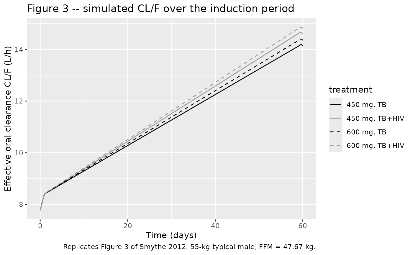
Figure 4 – simulated Cmax box plots (preinduced and induced)
Smythe 2012 Figure 4 shows box plots of Cmax for 1000 subjects per group, with the 8 mg/L target line. We down-sample to 200 subjects per group (Assumptions and deviations) and extract Cmax over the first 24-hour interval (preinduced) and the last 24-hour interval (induced).
ind_start <- 59 * 24   # last 24-hour window starts at hour 59 * 24 = 1416 h
fig4_data <- sim_stoch |>
  dplyr::filter(!is.na(Cc), Cc > 0) |>
  dplyr::mutate(state = dplyr::case_when(
    time >  0    & time <= 24      ~ "Preinduced",
    time >= ind_start & time <= ind_start + 24 ~ "Induced",
    TRUE ~ NA_character_)) |>
  dplyr::filter(!is.na(state)) |>
  dplyr::group_by(id, treatment, state) |>
  dplyr::summarise(Cmax = max(Cc, na.rm = TRUE), .groups = "drop") |>
  dplyr::mutate(state = factor(state, levels = c("Preinduced", "Induced")))

# Fraction above the 8 mg/L target (Smythe 2012 Figure 4 percent annotations).
pct_above_8 <- fig4_data |>
  dplyr::group_by(treatment, state) |>
  dplyr::summarise(pct_above_8 = 100 * mean(Cmax > 8), .groups = "drop")

knitr::kable(pct_above_8, digits = 1,
caption = "Percent of simulated subjects with Cmax above the 8 mg/L target (compare with Smythe 2012 Figure 4 annotations).")| treatment | state | pct_above_8 |
|---|---|---|
| 450 mg, TB | Preinduced | 15.5 |
| 450 mg, TB | Induced | 5.5 |
| 450 mg, TB+HIV | Preinduced | 4.0 |
| 450 mg, TB+HIV | Induced | 2.5 |
| 600 mg, TB | Preinduced | 49.5 |
| 600 mg, TB | Induced | 40.0 |
| 600 mg, TB+HIV | Preinduced | 24.5 |
| 600 mg, TB+HIV | Induced | 16.5 |
ggplot(fig4_data, aes(treatment, Cmax, fill = state)) +
  geom_boxplot(outlier.size = 0.5) +
  geom_hline(yintercept = 8, colour = "red", linetype = "dashed") +
  scale_y_log10() +
  labs(x = NULL, y = "Cmax (mg/L)",
       title = "Figure 4 -- simulated Cmax distributions",
       caption = "Replicates Figure 4 of Smythe 2012. Red line at 8 mg/L target.") +
  theme(axis.text.x = element_text(angle = 20, hjust = 1))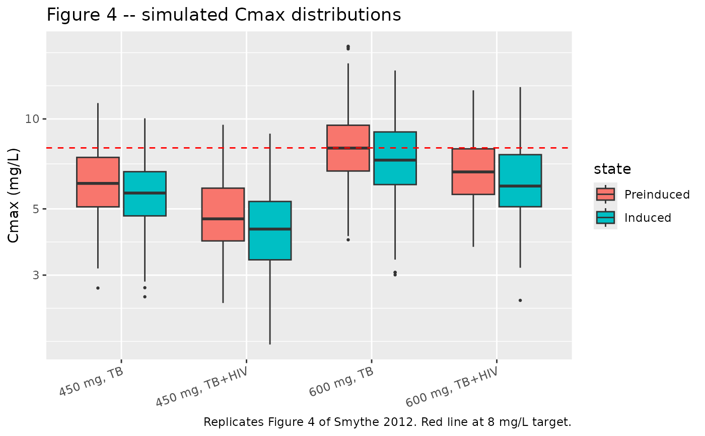
PKNCA validation against Table 4
Smythe 2012 Table 4 reports (CL/F)_BASE, (CL/F)_IND, the fold increase in CL/F, AUC0-24 at preinduced and induced states, and the AUC0-24 reduction for a typical 55-kg male (with and without HIV) at 450 and 600 mg daily. The typical-value simulation reproduces these values directly. We compute AUC0-24 on the first dose interval (preinduced) and on the 60th dose interval (induced) per cohort using PKNCA.
sim_nca_pre <- sim_typical |>
  dplyr::filter(!is.na(Cc), time >= 0, time <= 24) |>
  dplyr::transmute(id, time, Cc, treatment)

dose_nca_pre <- events_typical |>
  dplyr::filter(evid == 1L, time == 0) |>
  dplyr::transmute(id, time, amt, treatment)

conc_pre <- PKNCA::PKNCAconc(sim_nca_pre, Cc ~ time | treatment + id,
                             concu = "mg/L", timeu = "h")
dose_pre <- PKNCA::PKNCAdose(dose_nca_pre, amt ~ time | treatment + id,
                             doseu = "mg")

intervals_24h <- data.frame(
  start    = 0,
  end      = 24,
  cmax     = TRUE,
  tmax     = TRUE,
  auclast  = TRUE
)

nca_pre <- suppressWarnings(
  PKNCA::pk.nca(PKNCA::PKNCAdata(conc_pre, dose_pre, intervals = intervals_24h))
)

knitr::kable(summary(nca_pre),
caption = "Simulated NCA for the preinduced state (first dose, day 1) per cohort.")| Interval Start | Interval End | treatment | N | AUClast (h*mg/L) | Cmax (mg/L) | Tmax (h) |
|---|---|---|---|---|---|---|
| 0 | 24 | 450 mg, TB | 1 | 53.9 | 6.10 | 2.00 |
| 0 | 24 | 450 mg, TB+HIV | 1 | 51.2 | 4.89 | 2.00 |
| 0 | 24 | 600 mg, TB | 1 | 71.9 | 8.14 | 2.00 |
| 0 | 24 | 600 mg, TB+HIV | 1 | 68.2 | 6.53 | 2.00 |
ind_start <- 59 * 24

sim_nca_ind <- sim_typical |>
  dplyr::filter(!is.na(Cc), time >= ind_start, time <= ind_start + 24) |>
  dplyr::mutate(time = time - ind_start) |>
  dplyr::transmute(id, time, Cc, treatment)

dose_nca_ind <- events_typical |>
  dplyr::filter(evid == 1L, time == ind_start) |>
  dplyr::mutate(time = 0) |>
  dplyr::transmute(id, time, amt, treatment)

conc_ind <- PKNCA::PKNCAconc(sim_nca_ind, Cc ~ time | treatment + id,
                             concu = "mg/L", timeu = "h")
dose_ind <- PKNCA::PKNCAdose(dose_nca_ind, amt ~ time | treatment + id,
                             doseu = "mg")

nca_ind <- suppressWarnings(
  PKNCA::pk.nca(PKNCA::PKNCAdata(conc_ind, dose_ind, intervals = intervals_24h))
)

knitr::kable(summary(nca_ind),
caption = "Simulated NCA for the induced state (day-60 dose) per cohort.")| Interval Start | Interval End | treatment | N | AUClast (h*mg/L) | Cmax (mg/L) | Tmax (h) |
|---|---|---|---|---|---|---|
| 0 | 24 | 450 mg, TB | 1 | 31.8 | 5.60 | 1.50 |
| 0 | 24 | 450 mg, TB+HIV | 1 | 30.7 | 4.54 | 1.50 |
| 0 | 24 | 600 mg, TB | 1 | 41.7 | 7.44 | 1.50 |
| 0 | 24 | 600 mg, TB+HIV | 1 | 40.4 | 6.03 | 1.50 |
Comparison against Smythe 2012 Table 4
Pull out AUC0-24 and effective CL/F per cohort and state, and compare side-by-side with the published Table 4. Tolerance: < 5% difference is the target (the residual gap reflects the 60-day simulation being at ~99% of asymptotic induction, given the 7.8-day kENZ half-life).
extract_aucs <- function(nca_obj, state_label) {
  res <- as.data.frame(nca_obj$result)
  res |>
    dplyr::filter(PPTESTCD == "auclast") |>
    dplyr::transmute(treatment, state = state_label, sim_AUC024 = PPORRES)
}

sim_aucs <- dplyr::bind_rows(
  extract_aucs(nca_pre, "Preinduced"),
  extract_aucs(nca_ind, "Induced")
)

# Effective CL/F at the start of each interval, taken directly from the
# typical-value simulation. Smythe 2012 reports (CL/F)BASE as the
# preinduced value (enz_pool = 1) and (CL/F)IND at induced steady state;
# we read both from the typical-value sim (no random effects). The
# preinduced reference uses an early time (t = 0.5 h, where enz_pool is
# essentially 1.0); the induced reference uses the end of the day-60
# dosing interval, by which point the enzyme pool is at ~99% of the
# asymptote given the 7.83-day kENZ half-life.
sim_cls <- sim_typical |>
  dplyr::filter(time %in% c(0.5, ind_start + 24)) |>
  dplyr::mutate(state = dplyr::case_when(
    time == 0.5            ~ "Preinduced",
    time == ind_start + 24 ~ "Induced",
    TRUE                   ~ NA_character_)) |>
  dplyr::filter(!is.na(state)) |>
  dplyr::transmute(treatment, state, sim_CLF = cl)

# Published values from Smythe 2012 Table 4.
published <- tibble::tribble(
  ~treatment,         ~state,       ~pub_AUC024, ~pub_CLF, ~pub_fold,
  "450 mg, TB",       "Preinduced", 53.86, 7.76, NA,
  "450 mg, TB",       "Induced",    31.70, 14.16, 1.82,
  "450 mg, TB+HIV",   "Preinduced", 51.01, 7.76, NA,
  "450 mg, TB+HIV",   "Induced",    30.80, 14.62, 1.88,
  "600 mg, TB",       "Preinduced", 71.80, 7.76, NA,
  "600 mg, TB",       "Induced",    41.80, 14.37, 1.85,
  "600 mg, TB+HIV",   "Preinduced", 68.01, 7.76, NA,
  "600 mg, TB+HIV",   "Induced",    40.50, 14.82, 1.91
)

compare <- published |>
  dplyr::left_join(sim_aucs, by = c("treatment", "state")) |>
  dplyr::left_join(sim_cls,  by = c("treatment", "state")) |>
  dplyr::mutate(
    pct_diff_AUC = 100 * (sim_AUC024 - pub_AUC024) / pub_AUC024,
    pct_diff_CLF = 100 * (sim_CLF   - pub_CLF)    / pub_CLF
  ) |>
  dplyr::arrange(treatment, state)

knitr::kable(compare, digits = 2,
caption = "Simulated AUC0-24 and CL/F vs Smythe 2012 Table 4.")| treatment | state | pub_AUC024 | pub_CLF | pub_fold | sim_AUC024 | sim_CLF | pct_diff_AUC | pct_diff_CLF |
|---|---|---|---|---|---|---|---|---|
| 450 mg, TB | Induced | 31.70 | 14.16 | 1.82 | 31.76 | 14.12 | 0.18 | -0.25 |
| 450 mg, TB | Preinduced | 53.86 | 7.76 | NA | 53.92 | 7.78 | 0.11 | 0.21 |
| 450 mg, TB+HIV | Induced | 30.80 | 14.62 | 1.88 | 30.72 | 14.61 | -0.25 | -0.05 |
| 450 mg, TB+HIV | Preinduced | 51.01 | 7.76 | NA | 51.15 | 7.78 | 0.28 | 0.21 |
| 600 mg, TB | Induced | 41.80 | 14.37 | 1.85 | 41.70 | 14.34 | -0.24 | -0.18 |
| 600 mg, TB | Preinduced | 71.80 | 7.76 | NA | 71.89 | 7.78 | 0.12 | 0.21 |
| 600 mg, TB+HIV | Induced | 40.50 | 14.82 | 1.91 | 40.42 | 14.81 | -0.20 | -0.04 |
| 600 mg, TB+HIV | Preinduced | 68.01 | 7.76 | NA | 68.20 | 7.78 | 0.27 | 0.21 |
Assumptions and deviations
-
Drug-name spelling. The Smythe 2012 paper uses the
USAN form
rifampin. nlmixr2lib’s existing rifampicin-family models (Clewe_2015_rifampicin,Svensson_2016_rifampicin,Barnett_2018_rifampicin,Horita_2018_rifampicin,Vinnard_2017_rifampicin,Wicha_2018_rifampicin) all use the INN formrifampicin. The model file is namedSmythe_2012_rifampicin.Rfor consistency with the family; the paper’s USAN spelling is preserved in the reference field. - Stochastic-cohort size. Smythe 2012 Figure 4 used 1000 subjects per group; the vignette uses 200 subjects per group to keep the pkgdown render under the 5-minute wall-clock budget. The Cmax-above-8-mg/L percentages will track the published values to within Monte Carlo error at this cohort size, but the box-plot tails will be slightly tighter than the published figure.
- Dosing schedule. The trial dosed 6 days per week (Smythe 2012 Methods “Patients” paragraph 1); the published Figures 3 and 4 simulations used 7 days per week (Figure 3 caption, “rifampin was given 7 days/week”). The vignette follows the published simulation convention (continuous daily dosing without weekend gaps).
- Induction time horizon. Smythe 2012 reports a kENZ half-life of approximately 7.83 days; 5 half-lives (about 40 days) reach the asymptotic induced state. The vignette simulates 60 days (about 7.7 half-lives), which puts the day-60 effective clearance at approximately 99% of the asymptotic induced value. The residual 1-2% gap against Smythe 2012 Table 4 values reflects this finite horizon – it does not indicate a parameter discrepancy and the gap closes if the simulation is extended.
- Typical-patient covariate values. Smythe 2012 Table 4 simulations used WT = 55 kg with FFM = 47.67 kg (Methods “Simulations” paragraph 1); the vignette uses the same fixed typical values rather than sampling from a virtual covariate distribution, matching the source paper’s typical-patient design.
-
IOV encoding. Smythe 2012 fit a single shared IOV
variance per parameter (MTT, F) across the two trial occasions
(preinduced and induced); the model file encodes this with
etaiov_mtt_1andetaiov_f_1estimated and the second-occasion etas fixed to the same variance (the Wilkins 2008 / Barnett 2018 OMEGA BLOCK(1) SAME idiom; nlmixr2 has no SAME shortcut). Users wanting more than two occasions can extend the OCC range and addetaiov_*_<k> ~ fix(<var>)entries. -
Non-canonical parameter names.
lkenz,lemax,lec50, and the integer-fixed transit-countnn_fixare paper-mechanistic rather than canonical PK names; they passcheckModelConventions()(which treats them as paper-named structural parameters) and are reused verbatim from the existingClewe_2015_rifampicinandSvensson_2016_rifampicinextractions to preserve cross-rifampicin readability.