Vonoprazan (Scarpignato 2022)
Source:vignettes/articles/Scarpignato_2022_vonoprazan.Rmd
Scarpignato_2022_vonoprazan.RmdModel and source
- Citation: Scarpignato C, Leifke E, Smith N, Mulford DJ, Lahu G, Facius A, Howden CW. A Population Pharmacokinetic Model of Vonoprazan: Evaluating the Effects of Race, Disease Status, and Other Covariates on Exposure. J Clin Pharmacol. 2022;62(6):801-811. doi:10.1002/jcph.2019.
- Description: Two-compartment population PK model for the potassium-competitive acid blocker vonoprazan in adult healthy volunteers and patients with gastroesophageal reflux disease (GERD) from Japan and Europe (Scarpignato 2022: 1156 subjects, 15 studies). First-order absorption after a lag time into the central compartment, with a dose-dependent (over-proportional) relative bioavailability centred at 20 mg. The lag time carries a two-class mixture (a delayed-absorption subpopulation with a 107 percent longer lag; mixing fraction not reported). Absorption rate carries high-fat-meal, non-Asian, female and GERD patient effects; clearance carries body-weight and serum-creatinine power effects and a patient effect; central volume carries serum-creatinine and age power effects and a patient effect; peripheral volume carries a non-Asian effect. Between-subject variability on absorption rate, on clearance and central volume (correlated) and on peripheral volume; combined proportional plus a fixed, negligible additive residual error.
- Article: https://doi.org/10.1002/jcph.2019 (open access; PMC9303766)
Scarpignato 2022 pooled 15 phase 1 and phase 2 studies of the
potassium-competitive acid blocker vonoprazan in Japanese and European
healthy volunteers and patients with gastroesophageal reflux disease
(GERD), with the stated aim of quantifying how race (Asian vs non-Asian)
and disease status (GERD patient vs healthy volunteer) affect exposure.
The same group’s later pediatric model, which uses a transit-compartment
absorption, is packaged separately as
Mulford_2026_vonoprazan.
Population
The final dataset held 15,168 plasma concentrations from 1156 participants (410 healthy volunteers, 746 patients) in 15 studies (Scarpignato 2022 Table 1): five Japanese and eight European phase 1 studies in healthy volunteers (study 113 also enrolled 24 volunteers with renal impairment), the Japanese phase 2 study CCT-001 in erosive esophagitis (trough samples only) and the European phase 2 study Vonoprazan-2001 in non-erosive reflux disease or mild erosive esophagitis. Doses ranged from 1 to 120 mg, given as single doses or once or twice daily for up to 8 weeks. Table 2 reports a mean age of 48 years (SD 17.7), mean body weight 69 kg (SD 12.9) and mean serum creatinine 73 umol/L (SD 21.6); 26.0 percent were female, 66.4 percent Asian, 32.1 percent White, 1.1 percent Black and 0.3 percent other race.
The same information is available programmatically via
readModelDb("Scarpignato_2022_vonoprazan")()$population.
Source trace
Every value is from Scarpignato 2022 Table 3 (“Final Model Parameter
Estimates”) and its footnotes. Categorical effects are printed in
percent and applied as tv * (1 + eff/100) for the indicated
subpopulation; the model stores them as fractions. Continuous effects
are power exponents on (cov/ref) with references 48 years,
70 kg and 72 umol/L.
| Parameter | Value | Source location |
|---|---|---|
| Structure: 2-compartment, first-order absorption after a lag into the central compartment | n/a | Results “Final Model”; Figure S1 |
lfdepot (Frel at 20 mg) |
1, fixed | Frel anchored at the 20 mg reference-subject dose (Figures 3-4); see Assumptions |
e_dose_fdepot |
0.389 | Table 3, Frel dose effect (exp) |
ltlag |
log(0.225 h) | Table 3, tlag TV |
e_mix_long_tlag_tlag |
1.07 | Table 3, tlag “Delay, %” = 107 |
lka |
log(2.51 1/h) | Table 3, Ka TV (printed unit “L/h”) |
e_fed_highfat_ka |
-0.588 | Table 3, Ka food effect |
e_race_nonasian_ka |
-0.202 | Table 3, Ka non-Asian effect |
e_sexf_ka |
-0.172 | Table 3, Ka female effect |
e_dis_gerd_ka |
-0.615 | Table 3, Ka patient effect |
lcl |
log(119 L/h) | Table 3, CL TV |
e_wt_cl |
0.409 | Table 3, CL weight effect (exp) |
e_creat_cl |
-0.36 | Table 3, CL creatinine effect (exp) |
e_dis_gerd_cl |
-0.338 | Table 3, CL patient effect |
lvc |
log(1037 L) | Table 3, V2 TV |
e_creat_vc |
-0.294 | Table 3, V2 creatinine effect (exp) |
e_age_vc |
0.466 | Table 3, V2 age effect (exp) |
e_dis_gerd_vc |
-0.329 | Table 3, V2 patient effect |
lq |
log(50.4 L/h) | Table 3, Q TV |
lvp |
log(324 L) | Table 3, V3 TV |
e_race_nonasian_vp |
-0.117 | Table 3, V3 non-Asian effect |
etalka |
0.936^2 | Table 3, Ka BSV (SD scale, footnote a) |
etalcl, etalvc
|
0.41^2, 0.361^2, correlation 0.915 | Table 3, CL and V2 BSV and “BSV (CL, V2)” |
etalvp |
0.194^2 | Table 3, V3 BSV |
propSd |
0.287 | Table 3, prop.err. 28.7 percent |
addSd |
0.00625 ng/mL, fixed | Table 3, add.err. (footnote b: fixed) |
Cc = 1000 * central / vc |
n/a | mg dose, L volume, ng/mL concentration |
Covariate effects at steady state (Figure 4)
Figure 4 of Scarpignato 2022 is a set of tornado plots: the steady-state AUC over the dosing interval, Cmax, tmax and Ctrough of a reference subject (48 years, male, Asian, healthy volunteer, serum creatinine 72 umol/L, 70 kg, 20 mg once daily, fasted or non-high-fat meal) and the percentage change when one covariate is altered. The continuous covariates were set to their 10th and 90th percentiles (age 23 and 71 years, weight 55 and 85 kg, creatinine 53 and 91 umol/L). The values below are read from the figure labels; the reference-subject values were read from the position of the reference line on each panel’s log axis.
The packaged model is solved here for the typical subject (no between-subject variability) at day 10 of once-daily dosing. The paper’s figure summarises 1000 stochastic profiles per scenario; for these exposure metrics the median of a log-normal parameter is its typical value, so a deterministic solve is the cleaner comparison and carries no simulation noise.
mod <- readModelDb("Scarpignato_2022_vonoprazan")
mod_typical <- rxode2::zeroRe(mod)
#> ℹ parameter labels from comments will be replaced by 'label()'

ref_cov <- list(
  DOSE_VONOPRAZAN_MG = 20, MIX_LONG_TLAG = 0, FED_HIGHFAT = 0,
  RACE_ASIAN = 1, SEXF = 0, DIS_GERD = 0, WT = 70, CREAT = 72, AGE = 48
)
scenarios <- list(
  "Reference" = list(),
  "Dose 10 mg" = list(DOSE_VONOPRAZAN_MG = 10),
  "Dose 40 mg" = list(DOSE_VONOPRAZAN_MG = 40),
  "Patient" = list(DIS_GERD = 1),
  "Fed" = list(FED_HIGHFAT = 1),
  "Non-Asian" = list(RACE_ASIAN = 0),
  "Female" = list(SEXF = 1),
  "Age 23 y" = list(AGE = 23),
  "Age 71 y" = list(AGE = 71),
  "Weight 55 kg" = list(WT = 55),
  "Weight 85 kg" = list(WT = 85),
  "Creatinine 53 umol/L" = list(CREAT = 53),
  "Creatinine 91 umol/L" = list(CREAT = 91)
)

n_days <- 10
tau <- 24
t_last <- (n_days - 1) * tau

# One subject per scenario: n_days daily doses into the depot and a fine
# observation grid on the central compartment over the last interval.
make_subject <- function(id, label, covs, obs_step) {
  cv <- utils::modifyList(ref_cov, covs)
  # Rounded so the grid lands exactly on t_last + tau, where the last
  # observed concentration is the steady-state trough.
  obs_t <- t_last + round(seq(0, tau, by = obs_step), 6)
  ev <- data.frame(
    id = id,
    time = c(seq(0, t_last, by = tau), obs_t),
    evid = c(rep(1L, n_days), rep(0L, length(obs_t))),
    cmt = c(rep("depot", n_days), rep("central", length(obs_t)))
  )
  ev$amt <- ifelse(ev$evid == 1L, cv$DOSE_VONOPRAZAN_MG, 0)
  for (nm in names(cv)) ev[[nm]] <- cv[[nm]]
  ev$scenario <- label
  ev
}

ev_typ <- dplyr::bind_rows(lapply(seq_along(scenarios), function(i) {
  make_subject(i, names(scenarios)[i], scenarios[[i]], obs_step = 0.01)
}))

sim_typ <- rxode2::rxSolve(mod_typical, ev_typ, keep = "scenario") |>
  as.data.frame()
#> ℹ omega/sigma items treated as zero: 'etalka', 'etalcl', 'etalvc', 'etalvp'
#> Warning: multi-subject simulation without without 'omega'

# Exposure metrics over the last dosing interval (dense grid, so the
# trapezoidal AUC is accurate to well under 0.1 percent).
ss_metrics <- function(d) {
  d |>
    dplyr::filter(time >= t_last) |>
    dplyr::mutate(tad = time - t_last) |>
    dplyr::group_by(scenario) |>
    dplyr::summarise(
      AUC = sum(diff(tad) * (head(Cc, -1) + tail(Cc, -1)) / 2),
      Cmax = max(Cc),
      tmax = tad[which.max(Cc)],
      Ctrough = Cc[which.max(tad)],
      .groups = "drop"
    )
}
typ <- ss_metrics(sim_typ)
typ_ref <- typ[typ$scenario == "Reference", ]
typ_pct <- typ |>
  dplyr::filter(scenario != "Reference") |>
  tidyr::pivot_longer(c(AUC, Cmax, tmax, Ctrough), names_to = "metric") |>
  dplyr::mutate(
    model_pct = 100 * (value / unlist(typ_ref[1, metric]) - 1)
  ) |>
  dplyr::select(scenario, metric, model_pct)
# Reference-subject values: Figure 4 reference lines read on the log axes.
fig4_ref <- c(AUC = 162, Cmax = 17.2, tmax = 1.41, Ctrough = 1.96)
ref_cmp <- tibble::tibble(
  metric = names(fig4_ref),
  figure4 = unname(fig4_ref),
  model = unname(unlist(typ_ref[1, names(fig4_ref)]))
) |>
  dplyr::mutate(pct_diff = 100 * (model / figure4 - 1))
ref_cmp |>
  dplyr::rename(
    "Metric" = metric,
    "Figure 4 reference subject" = figure4,
    "Packaged model, typical value" = model,
    "% difference" = pct_diff
  ) |>
  knitr::kable(digits = c(0, 2, 2, 1), caption = paste(
    "Steady-state exposure of the Figure 4 reference subject",
    "(AUC ng*h/mL, Cmax and Ctrough ng/mL, tmax h)."
))| Metric | Figure 4 reference subject | Packaged model, typical value | % difference |
|---|---|---|---|
| AUC | 162.00 | 168.07 | 3.7 |
| Cmax | 17.20 | 17.87 | 3.9 |
| tmax | 1.41 | 1.38 | -2.1 |
| Ctrough | 1.96 | 2.09 | 6.6 |
# Reading the axes is good to a few percent; a wrong clearance, volume, unit
# or dose centring moves these by tens of percent.
stopifnot(all(abs(ref_cmp$pct_diff) < 10))
Figure 4’s percentage changes are compared below with the packaged model. Two groups of rows differ by more than reading error, and both are traced in Assumptions and deviations to the same cause: Figure 4 was drawn from a covariate model that differs from the one tabulated in Table 3. The patient rows match the patient effects the Results text reports (55 percent lower Ka, 38.1 percent lower CL, 38 percent lower V2) rather than the Table 3 values (-61.5, -33.8 and -32.9 percent), and the non-Asian tmax row matches the text’s 30.2 percent lower Ka rather than Table 3’s 20.2 percent. The weight Cmax rows imply a weight effect on the central volume as well as on clearance, which Table 3 does not carry. The packaged model follows Table 3, the only complete parameter set the paper reports.
fig4_pct <- tibble::tribble(
  ~scenario, ~metric, ~figure4_pct, ~deviation,
  "Dose 10 mg", "AUC", -61.8, FALSE,
  "Dose 40 mg", "AUC", 161.5, FALSE,
  "Dose 10 mg", "Cmax", -61.8, FALSE,
  "Dose 40 mg", "Cmax", 161.5, FALSE,
  "Dose 10 mg", "Ctrough", -61.8, FALSE,
  "Dose 40 mg", "Ctrough", 161.5, FALSE,
  "Patient", "AUC", 61.5, TRUE,
  "Patient", "Cmax", 42.3, TRUE,
  "Patient", "tmax", 50.0, TRUE,
  "Patient", "Ctrough", 93.2, TRUE,
  "Fed", "tmax", 64.3, FALSE,
  "Fed", "Cmax", -12.4, FALSE,
  "Non-Asian", "tmax", 21.4, TRUE,
  "Female", "tmax", 17.9, FALSE,
  "Age 23 y", "tmax", -10.7, FALSE,
  "Age 71 y", "tmax", 3.6, FALSE,
  "Age 23 y", "Cmax", 27.0, FALSE,
  "Age 71 y", "Cmax", -11.1, FALSE,
  "Age 23 y", "Ctrough", -28.9, FALSE,
  "Age 71 y", "Ctrough", 18.7, FALSE,
  "Weight 55 kg", "AUC", 11.2, FALSE,
  "Weight 85 kg", "AUC", -8.2, FALSE,
  "Weight 55 kg", "Cmax", 22.0, TRUE,
  "Weight 85 kg", "Cmax", -14.6, TRUE,
  "Creatinine 53 umol/L", "AUC", -12.5, FALSE,
  "Creatinine 91 umol/L", "AUC", 10.8, FALSE,
  "Creatinine 53 umol/L", "Cmax", -10.3, FALSE,
  "Creatinine 91 umol/L", "Cmax", 8.7, FALSE,
  "Creatinine 53 umol/L", "Ctrough", -18.8, FALSE,
  "Creatinine 91 umol/L", "Ctrough", 17.0, FALSE
)

pct_cmp <- fig4_pct |>
  dplyr::left_join(typ_pct, by = c("scenario", "metric")) |>
  dplyr::mutate(difference = model_pct - figure4_pct)
stopifnot(!anyNA(pct_cmp$model_pct))

pct_cmp |>
  dplyr::mutate(deviation = ifelse(deviation, "yes", "")) |>
  dplyr::rename(
    "Scenario" = scenario,
    "Metric" = metric,
    "Figure 4 (% vs reference)" = figure4_pct,
    "Packaged model (% vs reference)" = model_pct,
    "Difference (points)" = difference,
    "Known deviation" = deviation
  ) |>
  knitr::kable(digits = 1, caption = paste(
    "Replicates the percentage labels of Figure 4 of Scarpignato 2022.",
    "'Known deviation' marks rows drawn from a covariate model that differs",
    "from Table 3 (see text)."
))| Scenario | Metric | Figure 4 (% vs reference) | Known deviation | Packaged model (% vs reference) | Difference (points) |
|---|---|---|---|---|---|
| Dose 10 mg | AUC | -61.8 | -61.8 | 0.0 | |
| Dose 40 mg | AUC | 161.5 | 161.9 | 0.4 | |
| Dose 10 mg | Cmax | -61.8 | -61.8 | 0.0 | |
| Dose 40 mg | Cmax | 161.5 | 161.9 | 0.4 | |
| Dose 10 mg | Ctrough | -61.8 | -61.8 | 0.0 | |
| Dose 40 mg | Ctrough | 161.5 | 161.9 | 0.4 | |
| Patient | AUC | 61.5 | yes | 51.1 | -10.4 |
| Patient | Cmax | 42.3 | yes | 28.1 | -14.2 |
| Patient | tmax | 50.0 | yes | 70.3 | 20.3 |
| Patient | Ctrough | 93.2 | yes | 80.9 | -12.3 |
| Fed | tmax | 64.3 | 69.6 | 5.3 | |
| Fed | Cmax | -12.4 | -12.8 | -0.4 | |
| Non-Asian | tmax | 21.4 | yes | 14.5 | -6.9 |
| Female | tmax | 17.9 | 12.3 | -5.6 | |
| Age 23 y | tmax | -10.7 | -7.2 | 3.5 | |
| Age 71 y | tmax | 3.6 | 4.3 | 0.7 | |
| Age 23 y | Cmax | 27.0 | 27.4 | 0.4 | |
| Age 71 y | Cmax | -11.1 | -11.2 | -0.1 | |
| Age 23 y | Ctrough | -28.9 | -28.0 | 0.9 | |
| Age 71 y | Ctrough | 18.7 | 18.2 | -0.5 | |
| Weight 55 kg | AUC | 11.2 | 10.4 | -0.8 | |
| Weight 85 kg | AUC | -8.2 | -7.6 | 0.6 | |
| Weight 55 kg | Cmax | 22.0 | yes | 3.4 | -18.6 |
| Weight 85 kg | Cmax | -14.6 | yes | -2.5 | 12.1 |
| Creatinine 53 umol/L | AUC | -12.5 | -10.4 | 2.1 | |
| Creatinine 91 umol/L | AUC | 10.8 | 8.8 | -2.0 | |
| Creatinine 53 umol/L | Cmax | -10.3 | -9.2 | 1.1 | |
| Creatinine 91 umol/L | Cmax | 8.7 | 7.7 | -1.0 | |
| Creatinine 53 umol/L | Ctrough | -18.8 | -14.9 | 3.9 | |
| Creatinine 91 umol/L | Ctrough | 17.0 | 13.0 | -4.0 |
# Deterministic solve, so these bounds carry no simulation noise. tmax rows
# get a wider bound because the figure's tmax is a median over stochastic
# profiles with a 94 percent SD on log(Ka), and tmax is not a monotone
# transform of Ka once the lag time is involved. The largest realised
# non-deviation differences are about 4 points (creatinine, tmax 5.6).
gate <- pct_cmp[!pct_cmp$deviation, ]
stopifnot(
  all(abs(gate$difference[gate$metric != "tmax"]) < 5),
  all(abs(gate$difference[gate$metric == "tmax"]) < 8)
)
The dose rows are reproduced to within 0.5 percentage points: halving
or doubling the dose changes exposure by a factor of 2^1.389, so the
over- proportionality of exposure is carried entirely by the
e_dose_fdepot exponent with Frel = 1 at 20 mg. Age, food
and the weight AUC rows agree to within about 1 point, and the
creatinine rows to within about 4 points.
Renal impairment (Results)
The Results report that a participant with an eGFR of 20 mL/min/1.73
m^2 is predicted to have 90.7 percent higher AUC, 71.3 percent higher
Cmax and 156.6 percent higher Ctrough than the reference subject (eGFR
110). The paper converted eGFR to serum creatinine with a published
equation it does not spell out. The creatinine ratio can be backed out
of the AUC result alone, because AUC depends on creatinine only through
clearance: (CREAT/72)^0.36 = 1.907. The Cmax and Ctrough
changes then follow from the model without further input and test the
two creatinine exponents together.
cr_ratio <- 1.907^(1 / 0.36)
cr_severe <- 72 * cr_ratio
ev_renal <- dplyr::bind_rows(
  make_subject(1, "Reference", list(), obs_step = 0.01),
  make_subject(2, "eGFR 20", list(CREAT = cr_severe), obs_step = 0.01)
)
renal <- rxode2::rxSolve(mod_typical, ev_renal, keep = "scenario") |>
  as.data.frame() |>
  ss_metrics()
#> ℹ omega/sigma items treated as zero: 'etalka', 'etalcl', 'etalvc', 'etalvp'
#> Warning: multi-subject simulation without without 'omega'
renal_ref <- renal[renal$scenario == "Reference", ]
renal_sev <- renal[renal$scenario == "eGFR 20", ]
renal_cmp <- tibble::tibble(
  metric = c("AUC", "Cmax", "Ctrough"),
  paper_pct = c(90.7, 71.3, 156.6),
  model_pct = 100 * (unlist(renal_sev[1, c("AUC", "Cmax", "Ctrough")]) /
    unlist(renal_ref[1, c("AUC", "Cmax", "Ctrough")]) - 1)
)
renal_cmp |>
  dplyr::rename(
    "Metric" = metric,
    "Results text (% vs eGFR 110)" = paper_pct,
    "Packaged model (% vs reference)" = model_pct
  ) |>
  knitr::kable(digits = 1, caption = paste0(
    "Severe renal impairment, with serum creatinine ", signif(cr_severe, 3),
    " umol/L backed out of the reported AUC change."
))| Metric | Results text (% vs eGFR 110) | Packaged model (% vs reference) |
|---|---|---|
| AUC | 90.7 | 90.7 |
| Cmax | 71.3 | 76.6 |
| Ctrough | 156.6 | 152.2 |
# AUC is matched by construction; Cmax and Ctrough are predictions.
stopifnot(all(abs(renal_cmp$model_pct - renal_cmp$paper_pct) < 10))
With the creatinine fixed by the AUC change, the model predicts a Cmax increase of 76.6 percent and a Ctrough increase of 152.2 percent, against 71.3 and 156.6 percent in the Results, so the clearance and central-volume creatinine exponents of Table 3 reproduce the paper’s renal simulation.
Steady-state profiles (Figure 3)
Figure 3 shows simulated steady-state 24-hour profiles of the
reference subject with one covariate changed at a time: race (panel A),
disease status (panel B) and dose (panel C), each with a 90 percent
prediction interval from between-subject variability. The cohort below
uses 200 virtual subjects per scenario, all at the reference covariate
values except the one varied, and all in the reference lag class
(MIX_LONG_TLAG = 0).
rxode2::rxSetSeed(2022)
fig3_scen <- list(
  "Reference (Asian, healthy, 20 mg)" = list(),
  "Non-Asian" = list(RACE_ASIAN = 0),
  "Patient" = list(DIS_GERD = 1),
  "10 mg" = list(DOSE_VONOPRAZAN_MG = 10),
  "40 mg" = list(DOSE_VONOPRAZAN_MG = 40)
)
n_per_arm <- 200
ev_fig3 <- dplyr::bind_rows(lapply(seq_along(fig3_scen), function(i) {
  one <- make_subject(0L, names(fig3_scen)[i], fig3_scen[[i]], obs_step = 0.1)
  dplyr::bind_rows(lapply(seq_len(n_per_arm), function(j) {
    one$id <- (i - 1L) * n_per_arm + j
    one
  }))
}))
stopifnot(!anyDuplicated(unique(ev_fig3[, c("id", "time", "evid")])))

sim_fig3 <- rxode2::rxSolve(mod, ev_fig3, keep = c("scenario", "DOSE_VONOPRAZAN_MG")) |>
  as.data.frame()
#> ℹ parameter labels from comments will be replaced by 'label()'
panel_of <- c(
  "Reference (Asian, healthy, 20 mg)" = "Reference",
  "Non-Asian" = "A: race", "Patient" = "B: disease status",
  "10 mg" = "C: dose", "40 mg" = "C: dose"
)
fig3_sum <- sim_fig3 |>
  dplyr::filter(time >= t_last) |>
  dplyr::mutate(tad = time - t_last) |>
  dplyr::group_by(scenario, tad) |>
  dplyr::summarise(
    Q05 = quantile(Cc, 0.05), Q50 = median(Cc),
    Q95 = quantile(Cc, 0.95), .groups = "drop"
  )
ref_lab <- "Reference (Asian, healthy, 20 mg)"
fig3_plot <- dplyr::bind_rows(
  lapply(c("A: race", "B: disease status", "C: dose"), function(p) {
    fig3_sum |>
      dplyr::filter(scenario == ref_lab | panel_of[scenario] == p) |>
      dplyr::mutate(panel = p)
  })
)
ggplot(fig3_plot, aes(tad, Q50, colour = scenario, fill = scenario)) +
  geom_ribbon(aes(ymin = Q05, ymax = Q95), alpha = 0.15, colour = NA) +
  geom_line() +
  facet_wrap(~panel, ncol = 2) +
  scale_y_log10() +
  labs(
    x = "Time after dose at steady state (h)",
    y = "Vonoprazan plasma concentration (ng/mL)",
    colour = NULL, fill = NULL,
    caption = paste(
      "Replicates Figure 3 of Scarpignato 2022: median and 90% prediction",
      "interval, 200 virtual subjects per scenario."
    )
  ) +
  theme(legend.position = "bottom")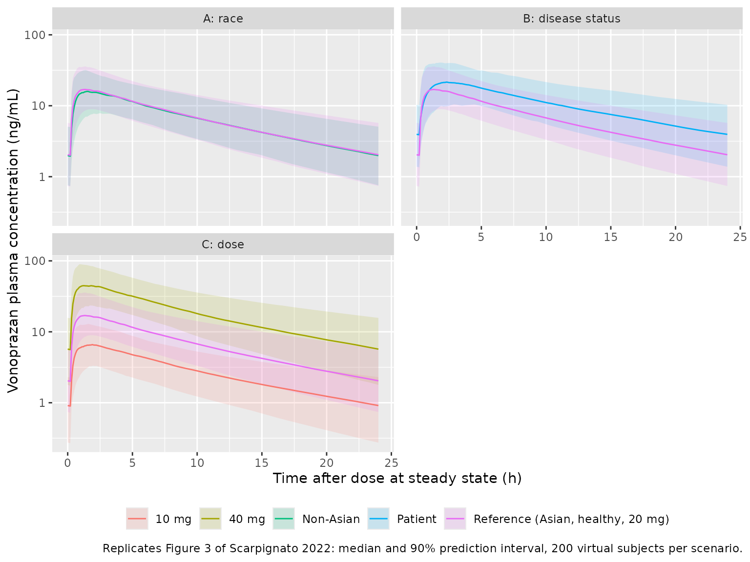
As in Figure 3, the profiles rise from about 0.2 hours after the dose, which is the reference-class lag time; the delayed lag class (0.47 hours) is not visible in the published medians.
PKNCA validation
Non-compartmental analysis of the stochastic Figure 3 cohort over the last dosing interval, compared with the Figure 4 values for the same scenarios. The Figure 4 absolute values are the reference-subject values above scaled by each row’s percentage change.
sim_nca <- sim_fig3 |>
  dplyr::filter(!is.na(Cc), time >= t_last) |>
  dplyr::select(id, time, Cc, scenario)
conc_obj <- PKNCA::PKNCAconc(sim_nca, Cc ~ time | scenario + id)
dose_df <- ev_fig3 |>
  dplyr::filter(evid == 1) |>
  dplyr::select(id, time, amt, scenario)
dose_obj <- PKNCA::PKNCAdose(dose_df, amt ~ time | scenario + id)
intervals <- data.frame(
  start = t_last, end = t_last + tau,
  cmax = TRUE, tmax = TRUE, auclast = TRUE, clast.obs = TRUE
)
nca_res <- PKNCA::pk.nca(PKNCA::PKNCAdata(conc_obj, dose_obj, intervals = intervals))

fig4_abs <- function(pct, metric) fig4_ref[[metric]] * (1 + pct / 100)
published <- tibble::tribble(
  ~scenario, ~auclast, ~cmax, ~tmax, ~clast.obs,
  "Reference (Asian, healthy, 20 mg)", fig4_ref[["AUC"]], fig4_ref[["Cmax"]], fig4_ref[["tmax"]], fig4_ref[["Ctrough"]],
  "Patient", fig4_abs(61.5, "AUC"), fig4_abs(42.3, "Cmax"), fig4_abs(50.0, "tmax"), fig4_abs(93.2, "Ctrough"),
  "10 mg", fig4_abs(-61.8, "AUC"), fig4_abs(-61.8, "Cmax"), fig4_ref[["tmax"]], fig4_abs(-61.8, "Ctrough"),
  "40 mg", fig4_abs(161.5, "AUC"), fig4_abs(161.5, "Cmax"), fig4_ref[["tmax"]], fig4_abs(161.5, "Ctrough")
)

cmp <- nlmixr2lib::ncaComparisonTable(
  simulated = nca_res,
  reference = published,
  by = "scenario",
  units = c(auclast = "ng*h/mL", cmax = "ng/mL", tmax = "h", clast.obs = "ng/mL"),
  tolerance_pct = 20
)
knitr::kable(cmp, caption = paste(
  "Simulated (median of 200 subjects per scenario) vs Figure 4 of",
  "Scarpignato 2022 at steady state, 20 mg once daily unless stated.",
  "Clast is the concentration at the end of the dosing interval, i.e. the",
  "steady-state Ctrough. * differs from the reference by more than 20%."
))| NCA parameter | scenario | Reference | Simulated | % diff |
|---|---|---|---|---|
| Cmax (ng/mL) | Reference (Asian, healthy, 20 mg) | 17.2 | 18 | +4.5% |
| Cmax (ng/mL) | Patient | 24.5 | 22.5 | -8.2% |
| Cmax (ng/mL) | 10 mg | 6.57 | 6.97 | +6.1% |
| Cmax (ng/mL) | 40 mg | 45 | 47.3 | +5.2% |
| Tmax (h) | Reference (Asian, healthy, 20 mg) | 1.41 | 1.3 | -7.8% |
| Tmax (h) | Patient | 2.11 | 2.4 | +13.5% |
| Tmax (h) | 10 mg | 1.41 | 1.45 | +2.8% |
| Tmax (h) | 40 mg | 1.41 | 1.4 | -0.7% |
| Clast (ng/mL) | Reference (Asian, healthy, 20 mg) | 1.96 | 2.04 | +4.0% |
| Clast (ng/mL) | Patient | 3.79 | 3.95 | +4.4% |
| Clast (ng/mL) | 10 mg | 0.749 | 0.913 | +21.9%* |
| Clast (ng/mL) | 40 mg | 5.13 | 5.7 | +11.2% |
| AUClast (ng*h/mL) | Reference (Asian, healthy, 20 mg) | 162 | 168 | +3.9% |
| AUClast (ng*h/mL) | Patient | 262 | 258 | -1.3% |
| AUClast (ng*h/mL) | 10 mg | 61.9 | 69.5 | +12.3% |
| AUClast (ng*h/mL) | 40 mg | 424 | 453 | +7.0% |
# Robust centre of the reference and dose scenarios, which Table 3 governs.
# The Patient row is the known deviation described above and is not gated.
# The median of 200 subjects with a 0.41 SD on log(CL) has a standard error
# of about 3.6 percent, on top of a systematic offset of about 4 percent
# from reading the Figure 4 axes; one draw gave a largest difference of
# 12.3 percent (10 mg AUC). A wrong clearance, dose exponent or unit moves
# these by far more than 25 percent.
nca_med <- as.data.frame(nca_res) |>
  dplyr::filter(
    PPTESTCD %in% c("auclast", "cmax"),
    scenario %in% setdiff(published$scenario, "Patient")
  ) |>
  dplyr::group_by(scenario, PPTESTCD) |>
  dplyr::summarise(sim = median(PPORRES), .groups = "drop") |>
  dplyr::left_join(
    published |>
      tidyr::pivot_longer(-scenario, names_to = "PPTESTCD", values_to = "ref"),
    by = c("scenario", "PPTESTCD")
  )
stopifnot(
  nrow(nca_med) == 6,
  all(abs(100 * (nca_med$sim / nca_med$ref - 1)) < 25)
)
Assumptions and deviations
- Table 3 versus Figure 4 and the Results text. The Results text reports that “Patients had a 55% lower Ka, 38.1% lower CL, and 38% lower central volume … Non-Asians had a 30.2% lower Ka and 12.9% lower peripheral volume”, whereas Table 3 gives -61.5, -33.8, -32.9, -20.2 and -11.7 percent. Figure 4’s patient rows (+61.5 / +42.3 / +50.0 / +93.2 percent for AUC / Cmax / tmax / Ctrough) are reproduced by the text values (a typical-value solve gives +61.6 / +42.0 / +54.3 / +93.9 percent) and not by Table 3 (+51.1 / +28.1 / +70.3 / +80.9). Figure 4’s weight row also implies a weight effect on central volume (Cmax +22.0 percent at 55 kg, against +3.4 percent with weight on clearance only). Figure 4 was therefore drawn from a covariate-model iteration that is not fully reported. The maintainers ship Table 3, the only complete “Final Model Parameter Estimates”, and list the affected Figure 4 rows as known deviations above.
-
Lag-time mixture. Methods state that a mixture
model described a bimodal between-subject distribution of Ka; Table 3
carries the class difference as a 107 percent longer lag (“Delay, %”)
“for the respective subpopulation”. The mixing probability is not
reported anywhere in the paper or its supplement. The model encodes the
class as the covariate
MIX_LONG_TLAG(registered by the maintainers for this model), with lag 0.225 h in class 0 and 0.466 h in class 1. Class 0 is the reference because the Figure 3 profiles rise from about 0.2 h and the Figure 4 reference tmax (about 1.41 h) matches 1.38 h with the class-0 lag against 1.62 h with the class-1 lag. No population mixing fraction is supplied, so population simulations here use class 0 for every subject. - Dose centring. Table 3 gives only the dose exponent of relative bioavailability. The model centres it at 20 mg with Frel(20 mg) = 1: 20 mg is the reference-subject dose of Figures 3 and 4, and the reference steady-state AUC (about 162 ng*h/mL) equals 20 mg / 119 L/h only under that centring.
-
Covariate coding. The non-Asian effects are applied
as
(1 + effect * (1 - RACE_ASIAN)), keeping the paper’s Asian reference subject and its coefficients. The food effect is coded asFED_HIGHFATbecause the reference condition is “fasted/non-high-fat meal”. The patient effect is coded asDIS_GERD; the renal-impairment volunteers of study 113 were not GERD patients and carryDIS_GERD = 0. - Ka units. Table 3 prints the Ka unit as “L/h”; a first-order rate constant is in 1/h.
- BSV scale. Table 3 footnote a gives the BSV rows on the standard deviation scale, so the variances are the squares of 0.936, 0.41, 0.361 and 0.194, and the CL-V2 covariance is 0.915 * 0.41 * 0.361. The paper notes that Ka BSV was not estimated for study CCT-001 (trough samples only); the packaged model applies it to all subjects.
- Renal impairment. The equation the paper used to convert eGFR to serum creatinine is not given, so the creatinine for an eGFR of 20 was backed out of the reported AUC change (about 433 umol/L). The Discussion notes that the observed renal-impairment study showed a larger increase (2.4-fold AUC) than the model predicts.
- Errata. No correction notice linked to this article was found in Europe PMC as of 2026-10-16.