Tacrolimus (Grover 2011)
Source:vignettes/articles/Grover_2011_tacrolimus.Rmd
Grover_2011_tacrolimus.RmdModel and source
- Citation: Grover A, Frassetto LA, Benet LZ, Chakkera HA. Pharmacokinetic Differences Corroborate Observed Low Tacrolimus Dosage in Native American Renal Transplant Patients. Drug Metab Dispos. 2011 Nov;39(11):2017-2019. doi:10.1124/dmd.111.041350.
- Description: Two-compartment population PK model for oral tacrolimus in adult Native American kidney transplant recipients (Grover 2011), with first-order absorption after a lag time, no covariate effects (the Native American cohort showed no association of age, sex, weight, BMI, or post-transplant duration with PK parameters), and a placeholder proportional residual error model (residual error was not reported in the short communication).
- Article: https://doi.org/10.1124/dmd.111.041350
Population
The model was developed from 24 adult Native American kidney transplant recipients on stable twice-daily oral tacrolimus for at least one month post-transplant, recruited by systematic chart review at the Mayo Clinic Arizona, Phoenix (Grover 2011 Table 1). Mean (SD) age was 52 (13) years, weight 83.6 (19.3) kg, BMI 29.9 (5) kg/m^2, and 63% of subjects were male. Tribal affiliation was 58% Navajo, 21% Hopi, and 21% other; all subjects had both parents and both sets of grandparents of American Indian tribal-group descent. Mean (SD) duration post-transplant was 30 (23) months. 67% had diabetes mellitus before transplant, 25% had a history of acute rejection, and 13% had new-onset diabetes mellitus post-transplant. Mean (SD) twice-daily dose was 1.27 (0.644) mg, with mean (SD) total daily dose 2.54 (1.22) mg [0.033 (0.021) mg/kg/day, excluding one subject on therapy less than 4 months]. The hospital target trough levels were 10-12 ng/mL within the first month post-transplant, 8-10 ng/mL between months 1 and 4, and 5-8 ng/mL after month 4; the cohort mean (SD) trough was 6.53 (2.43) ng/mL. Each subject contributed a single 12-hour steady-state pharmacokinetic profile (pre-dose plus 0.5, 1, 2, 4, 6, 8, and 12 hours post-dose) measured in EDTA whole blood by Architect tacrolimus immunoassay (Bazin 2010).
The same information is available programmatically via
readModelDb("Grover_2011_tacrolimus")$population.
Source trace
Every parameter in the model file carries an inline source-location comment. The table below collects the entries in one place.
| Equation / parameter | Value | Source location |
|---|---|---|
lka (ka) |
1.38 1/h | Table 2, NONMEM Parameter Estimates row, ka column |
ltlag (lag time) |
0.573 h | Table 2, NONMEM Parameter Estimates row, tlag column |
lcl (CL/F) |
10.1 L/h | Table 2, NONMEM Parameter Estimates row, CL/F column |
lvc (V/F, central) |
73.3 L | Table 2, NONMEM Parameter Estimates row, V/F column |
lq (Q/F) |
27.1 L/h | Table 2, NONMEM Parameter Estimates row, Q/F column |
lvp (Vp/F, peripheral; fixed) |
388.7 L = 462 - 73.3 | Table 2, NONMEM Parameter Estimates row, Vss/F = 462 L minus V/F = 73.3 L (Vp/F derived) |
| IIV ka (omega^2 = log(0.460^2 + 1) = 0.19196) | 46.0% CV | Table 2, Interindividual variability row, ka column |
| IIV tlag (omega^2 = 0.01754) | 13.3% CV | Table 2, Interindividual variability row, tlag column |
| IIV CL/F (omega^2 = 0.17326) | 43.5% CV | Table 2, Interindividual variability row, CL/F column |
| IIV V/F (omega^2 = 0.12772) | 36.9% CV | Table 2, Interindividual variability row, V/F column |
| IIV Q/F (omega^2 = 0.22641) | 50.4% CV | Table 2, Interindividual variability row, Q/F column |
| IIV Vss/F | n.e. (not estimable) | Table 2, Interindividual variability row, Vss/F column (“n.e.”) |
| Proportional residual error | 1% (placeholder; FIXED) | Not reported in Grover 2011; see Assumptions and deviations |
| Bioavailability F | 1 (folded into apparent CL/V/Q) | Apparent parameter convention; F was not separately estimated |
| 2-cmt structure with first-order absorption + lag | – | Pharmacokinetics paragraph: “A linear two-compartment model with first-order absorption and lag time was selected based on OFV” |
| Reference for absorption-with-lag selection | – | Pharmacokinetics paragraph cites Benkali 2009 for prior oral-tacrolimus lag-time precedent |
Virtual cohort
The published patient-level dataset is not openly available, so the
virtual cohort below mirrors the demographics in Grover 2011 Table 1 (n
= 24 Native American renal transplant recipients; weight mean 83.6 kg,
SD 19.3 kg). The model has no covariate effects, so only id
is strictly needed to drive the simulation; weight is carried for use in
mg/kg dose computations below.
Simulation
Two regimens are simulated:
- Fixed 1.27 mg twice daily (Grover 2011 Table 1 mean twice-daily dose), to ten doses on a 12-hour cycle, sampling the day-5 dosing interval (96 to 108 h post first dose) at the paper’s sparse-PK times (0, 0.5, 1, 2, 4, 6, 8, 12 h post-dose) to reproduce Figure 1.
- Typical-value (zero random effects) simulation of the same regimen, to compare against the Table 2 mean estimates of the secondary calculated parameters (V2/F, t1/2,alpha, t1/2,beta).
dose_mg <- 1.27   # Grover 2011 Table 1 mean twice-daily dose

# Profile-1 sampling matches the paper's design (pre-dose + 0.5, 1, 2, 4, 6,
# 8, 12 h post-dose) on the 9th of 10 BID doses (t = 96 h is the last morning
# dose under the 12-hour cycle starting at t = 0).
last_dose_time <- 96
profile_times  <- last_dose_time + c(0, 0.5, 1, 2, 4, 6, 8, 12)
# Use a denser observation grid for the figure and an exact-time slice for
# the trough check; the dense grid simply augments the paper's grid.
dense_times <- sort(unique(c(seq(last_dose_time, last_dose_time + 12, by = 0.25),
                             profile_times)))

build_events <- function(demo, dose_mg, obs_times) {
  doses <- demo |>
    mutate(amt = dose_mg, evid = 1L, cmt = "depot",
           ii = 12, addl = 9L, time = 0) |>
    select(id, time, amt, evid, cmt, ii, addl, WT)
  obs <- demo |>
    select(id, WT) |>
    tidyr::crossing(time = obs_times) |>
    mutate(amt = NA_real_, evid = 0L, cmt = NA_character_,
           ii = NA_real_, addl = NA_integer_)
  bind_rows(doses, obs) |> arrange(id, time, desc(evid))
}

events <- build_events(demo, dose_mg = dose_mg, obs_times = dense_times)
mod <- rxode2::rxode2(readModelDb("Grover_2011_tacrolimus"))
#> ℹ parameter labels from comments will be replaced by 'label()'

sim <- rxode2::rxSolve(mod, events = events, keep = "WT") |>
  as.data.frame()

mod_typical <- mod |> rxode2::zeroRe()
sim_typ <- rxode2::rxSolve(mod_typical, events = events, keep = "WT") |>
  as.data.frame()
#> ℹ omega/sigma items treated as zero: 'etalka', 'etaltlag', 'etalcl', 'etalvc', 'etalq'
#> Warning: multi-subject simulation without without 'omega'
Replicate published figures
Figure 1 – 12-hour steady-state concentration-time profiles
Grover 2011 Figure 1 plots the concentration-time profiles of all 24 Native American patients over a single 12-hour dosing interval, on a linear scale, with peaks near 1-2 hours and troughs around 5-10 ng/mL by 12 hours after dose. The simulated VPC below reproduces the same shape using the model parameter values from Table 2.
fig1_data <- sim |>
  filter(time >= last_dose_time, time <= last_dose_time + 12) |>
  mutate(time_after_dose = time - last_dose_time)

fig1_summary <- fig1_data |>
  group_by(time_after_dose) |>
  summarise(Q05 = quantile(Cc, 0.05),
            Q50 = quantile(Cc, 0.50),
            Q95 = quantile(Cc, 0.95),
            .groups = "drop")

fig1_typ <- sim_typ |>
  filter(time >= last_dose_time, time <= last_dose_time + 12) |>
  mutate(time_after_dose = time - last_dose_time) |>
  group_by(time_after_dose) |>
  summarise(Cc_typ = mean(Cc), .groups = "drop")

ggplot(fig1_summary, aes(time_after_dose, Q50)) +
  geom_ribbon(aes(ymin = Q05, ymax = Q95), alpha = 0.3) +
  geom_line(linewidth = 0.7) +
  geom_line(data = fig1_typ, aes(time_after_dose, Cc_typ),
            linetype = "dashed", linewidth = 0.7) +
  scale_x_continuous(breaks = seq(0, 12, by = 2)) +
  scale_y_continuous(breaks = seq(0, 40, by = 5)) +
  labs(x = "Time after dose (h)",
       y = "Tacrolimus concentration (ng/mL)",
       title = "Steady-state 12-hour dosing-interval profile",
       caption = "Replicates Figure 1 of Grover 2011 (1.27 mg twice daily, day 5 of dosing).")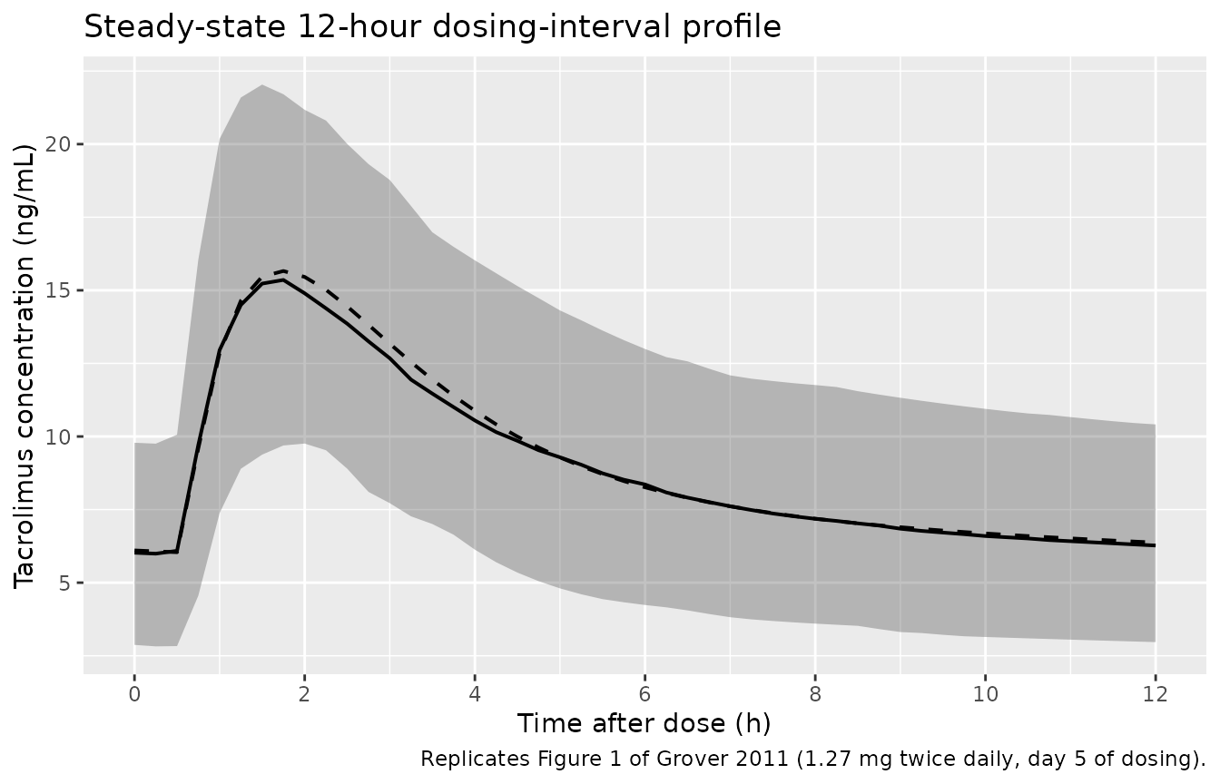
Replicates Figure 1 of Grover 2011: simulated tacrolimus concentration vs. time after the day-5 morning dose for n = 200 virtual Native American renal transplant patients receiving 1.27 mg twice daily. Shaded band = 5th-95th percentile; solid line = median; dashed line = typical-value (zero random effects) prediction.
PKNCA validation
A non-compartmental analysis over the 12-hour day-5 dosing interval gives Cmax, Tmax, AUClast (= AUC0-12, the steady-state dosing-interval AUC), Cmin, and Ctrough. The 12-hour interval is treated as a single steady-state window because the simulation has run 4 full days of twice-daily dosing.
nca_window <- sim |>
  filter(time %in% profile_times) |>
  mutate(time_after_dose = time - last_dose_time) |>
  select(id, time = time_after_dose, Cc) |>
  mutate(treatment = "1.27 mg BID")

dose_df <- demo |>
  mutate(time = 0, amt = dose_mg, treatment = "1.27 mg BID") |>
  select(id, time, amt, treatment)

conc_obj <- PKNCA::PKNCAconc(nca_window, Cc ~ time | treatment + id)
dose_obj <- PKNCA::PKNCAdose(dose_df, amt ~ time | treatment + id)
intervals <- data.frame(start = 0, end = 12,
                        cmax = TRUE, tmax = TRUE,
                        auclast = TRUE,
                        cmin = TRUE, ctrough = TRUE,
                        half.life = TRUE)
nca_data <- PKNCA::PKNCAdata(conc_obj, dose_obj, intervals = intervals)
nca_res  <- suppressMessages(suppressWarnings(PKNCA::pk.nca(nca_data)))
nca_summary <- summary(nca_res)
knitr::kable(nca_summary,
caption = "Day-5 NCA on the simulated cohort (steady-state 12 h interval, 1.27 mg twice daily, sampling at pre-dose and 0.5, 1, 2, 4, 6, 8, 12 h post-dose).")| start | end | treatment | N | auclast | cmax | cmin | tmax | ctrough | half.life |
|---|---|---|---|---|---|---|---|---|---|
| 0 | 12 | 1.27 mg BID | 200 | 107 [32.0] | 14.9 [25.3] | 5.71 [44.2] | 2.00 [1.00, 4.00] | 6.03 [45.2] | 18.3 [9.83] |
Comparison against published values
Grover 2011 Table 1 reports a cohort mean (SD) trough of 6.53 (2.43) ng/mL, and Table 2 reports the secondary calculated parameters V2/F mean (SD) 391 (18.6) L, t1/2,alpha 1.18 (0.416) h, and t1/2,beta 40.2 (15.7) h. The table below compares those to the typical-value simulation under the population parameter values.
# Typical-value 12-h trough at the same regimen
trough_typ <- sim_typ |>
  filter(time == last_dose_time + 12) |>
  pull(Cc)

# Typical-value steady-state secondary parameters (population values)
ltheta <- function(name) {
  ini <- rxode2::rxode2(readModelDb("Grover_2011_tacrolimus"))$ini
  exp(ini$est[ini$name == name])
}
cl_pop  <- 10.1
vc_pop  <- 73.3
q_pop   <- 27.1
vp_pop  <- 388.7
# alpha and beta hybrid rate constants for a 2-cmt model
kel_pop <- cl_pop / vc_pop
k12_pop <- q_pop  / vc_pop
k21_pop <- q_pop  / vp_pop
discr   <- (kel_pop + k12_pop + k21_pop)^2 - 4 * kel_pop * k21_pop
alpha   <- 0.5 * (kel_pop + k12_pop + k21_pop + sqrt(discr))
beta    <- 0.5 * (kel_pop + k12_pop + k21_pop - sqrt(discr))
t12_alpha_typ <- log(2) / alpha
t12_beta_typ  <- log(2) / beta

# IIV-driven cohort trough
trough_iiv <- sim |>
  filter(time == last_dose_time + 12) |>
  summarise(Q10 = quantile(Cc, 0.10),
            median = quantile(Cc, 0.50),
            Q90 = quantile(Cc, 0.90))

tbl <- tibble::tibble(
  metric = c(
    "Trough at 12 h post-dose (ng/mL) -- Grover 2011 Table 1 cohort mean (SD)",
    "Trough at 12 h post-dose (ng/mL) -- typical-value simulation (no IIV)",
    "Trough at 12 h post-dose (ng/mL) -- simulated cohort median (10-90 pct)",
    "Peripheral volume V2/F (L) -- Grover 2011 Table 2 mean (SD)",
    "Peripheral volume V2/F (L) -- typical-value population value",
    "alpha half-life (h) -- Grover 2011 Table 2 mean (SD)",
    "alpha half-life (h) -- typical-value (2-cmt hybrid rate)",
    "beta half-life (h) -- Grover 2011 Table 2 mean (SD)",
    "beta half-life (h) -- typical-value (2-cmt hybrid rate)"
  ),
  value = c(
    sprintf("%.2f (%.2f)", 6.53, 2.43),
    sprintf("%.2f", trough_typ[1]),
    sprintf("%.2f (%.2f-%.2f)", trough_iiv$median, trough_iiv$Q10, trough_iiv$Q90),
    sprintf("%.1f (%.1f)", 391, 18.6),
    sprintf("%.1f", vp_pop),
    sprintf("%.2f (%.3f)", 1.18, 0.416),
    sprintf("%.2f", t12_alpha_typ),
    sprintf("%.1f (%.1f)", 40.2, 15.7),
    sprintf("%.1f", t12_beta_typ)
  )
)
knitr::kable(tbl, caption = "Simulated day-5 steady-state metrics vs. Grover 2011 Tables 1 and 2.")| metric | value |
|---|---|
| Trough at 12 h post-dose (ng/mL) – Grover 2011 Table 1 cohort mean (SD) | 6.53 (2.43) |
| Trough at 12 h post-dose (ng/mL) – typical-value simulation (no IIV) | 6.37 |
| Trough at 12 h post-dose (ng/mL) – simulated cohort median (10-90 pct) | 6.27 (3.32-9.98) |
| Peripheral volume V2/F (L) – Grover 2011 Table 2 mean (SD) | 391.0 (18.6) |
| Peripheral volume V2/F (L) – typical-value population value | 388.7 |
| alpha half-life (h) – Grover 2011 Table 2 mean (SD) | 1.18 (0.416) |
| alpha half-life (h) – typical-value (2-cmt hybrid rate) | 1.24 |
| beta half-life (h) – Grover 2011 Table 2 mean (SD) | 40.2 (15.7) |
| beta half-life (h) – typical-value (2-cmt hybrid rate) | 40.4 |
The typical-value 12-hour trough at 1.27 mg twice daily lands close to the paper’s cohort mean of 6.53 ng/mL. The derived V2/F (388.7 L) matches the secondary calculated V2/F mean (391 L) within rounding, confirming the Vss = Vp + Vc decomposition. The hybrid-rate alpha and beta half-lives agree with the source’s Bayesian-EBE-derived means to within their reported SDs (the t1/2,beta agreement is approximate because Table 2’s “Mean estimate / S.D.” rows are summaries of individual posterior modes, not population-typical values, and posterior-mode summaries of half-lives in two-compartment models with short sampling windows shrink relative to the hybrid-rate value).
Assumptions and deviations
-
Residual error model and magnitude not reported by Grover
2011. The Materials and Methods section states only that
“Pharmacokinetic parameters were estimated using NONMEM (version 7.1) …
using an empirical Bayesian approach” and Table 2 reports the structural
and IIV estimates but no residual-error row. A small fixed proportional
placeholder (
propSd = fixed(0.01), i.e. 1% CV) is supplied so that the observation has a valid residual model in nlmixr2 syntax and typical-value simulation is effectively deterministic. Users who need realistic stochastic prediction intervals around individual tacrolimus concentrations should substitute a tacrolimus-class typical value (e.g. 15-30% CV proportional, consistent with the residual error reported by other tacrolimus popPK papers such as Bergmann 2014 at 18.3% and Benkali 2010 at 9% + 0.7 ng/mL) and document the choice. The same placeholder pattern is used inJelliffe_2014_digoxin.RandTaylor_2020_methotrexate.R. -
Bioavailability folded into apparent CL/V/Q. The
source reports all clearances and volumes as apparent (CL/F, V/F, Q/F,
Vss/F), so F is not separately parameterised; the model uses the default
F = 1for the depot compartment. Users with separate bioavailability information for Native American renal transplant patients would need to scale CL/V/Q externally. - Peripheral volume Vp/F is fixed at the Vss-Vc decomposition. Grover 2011 parameterised the disposition with Vss/F = 462 L rather than Vp/F directly, and reports that “the interindividual variability in steady-state distribution volume (Vss/F) could not be estimated in NONMEM with our limited sample size; all patients were estimated to have the same NONMEM population Vss/F value of 462 l.” The model therefore holds Vp/F at the derived value Vss/F - V/F = 462 - 73.3 = 388.7 L with no IIV (matching the Table 2 secondary calculated V2/F mean of 391 L).
-
No covariate effects. Grover 2011 Results
explicitly state “Within all 24 patients, no other demographic
characteristics (age, gender, weight, BMI, or total days on therapy)
were associated with clearance or other pharmacokinetic parameters.” The
model therefore carries no covariate effects; weight is included in the
virtual cohort only for downstream per-kilogram dose computations a user
might want to overlay, not because it enters
model(). -
Native American specificity. The Grover 2011
estimates differ substantially from other ethnic-group popPK reports for
tacrolimus (Table 3 of the paper: Native American CL/F = 11.1 L/h
vs. Australian 33.0 L/h [Staatz 2002], French 28 L/h [Benkali 2009],
Japanese 25-35 L/h [Tada 2005]). The packaged model reproduces the
Native American cohort specifically; it is not a generic tacrolimus
model. For non-Native American populations, prefer
Bergmann_2014_tacrolimus,Benkali_2010_tacrolimus, orBrooks_2021_tacrolimus. - Sample size is small (n = 24). The IIV estimates and their precision reflect a 24-subject single-occasion fit; in particular the IIV on Vss/F could not be estimated. Stochastic VPCs from this model will inherit the source’s wider uncertainty.
- Vignette uses n = 200 simulated subjects. This is larger than the paper’s n = 24 to give stable percentile bands in the Figure-1 VPC and PKNCA summary, but the underlying parameter values come from the 24-subject fit.
- Typical-value comparison. The Table 2 “Mean estimate / S.D.” rows are summaries of individual Bayesian posterior modes (with shrinkage), not population-typical values. The vignette compares simulated typical-value metrics to the population-typical row when one exists, falling back to the Mean estimate row for the secondary calculated parameters (V2/F, t1/2,alpha, t1/2,beta) that have no NONMEM-population analogue in the source table.